Many common nuclides emit two or more photons from the same decay, often called a cascade. The initial decay (it could be α, β-, β+ or electron capture) populates an excited state in the daughter nucleus. This state will decay by photon emission or internal conversion to a less-excited state in the nucleus (which could be the ground state).
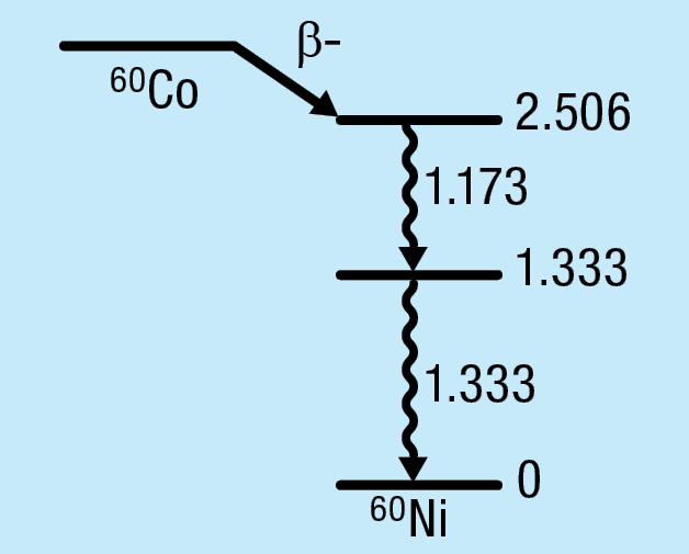
Figure 12-1 shows the decay schema of 60Co, where the sequential decays from the excited states can be seen.
Figure 12-1: The decay schema of 60Co decay.
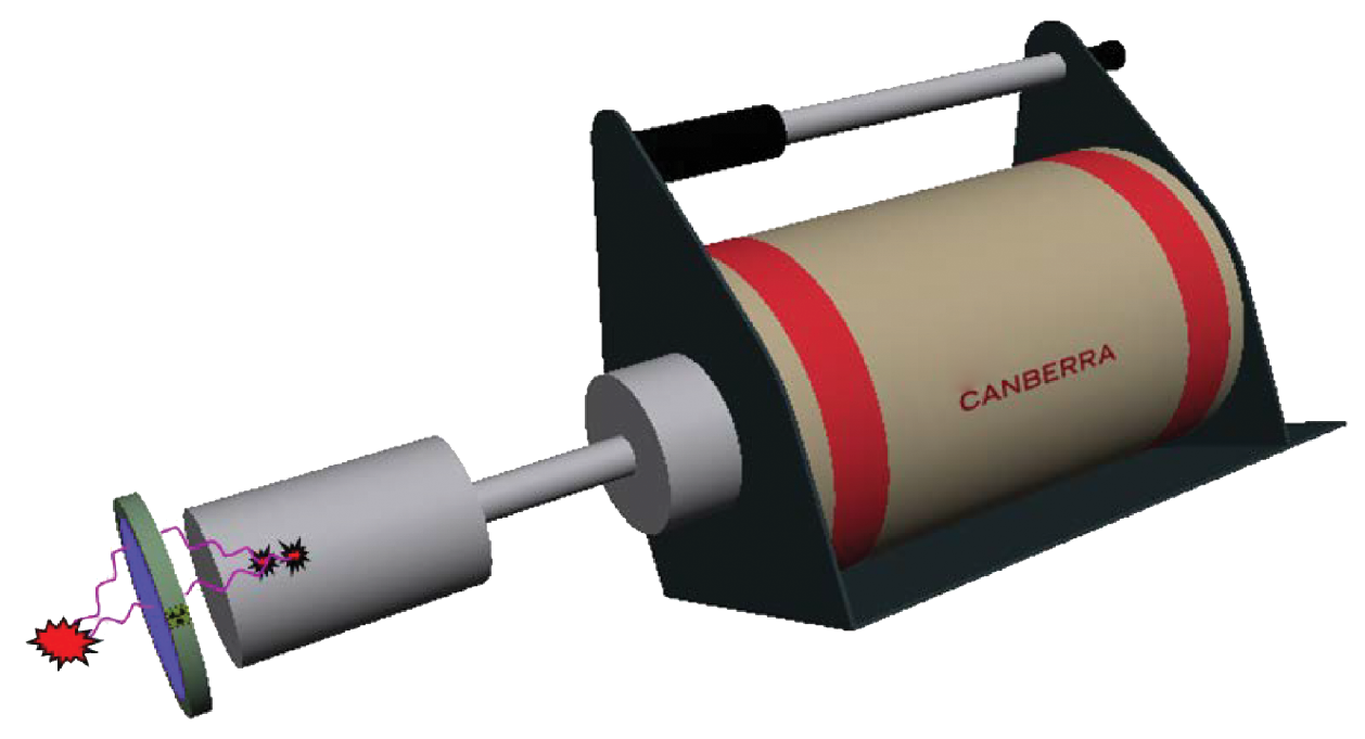
Figure 12-2: A decay emitting two photons and both of them depositing energy in the detector.
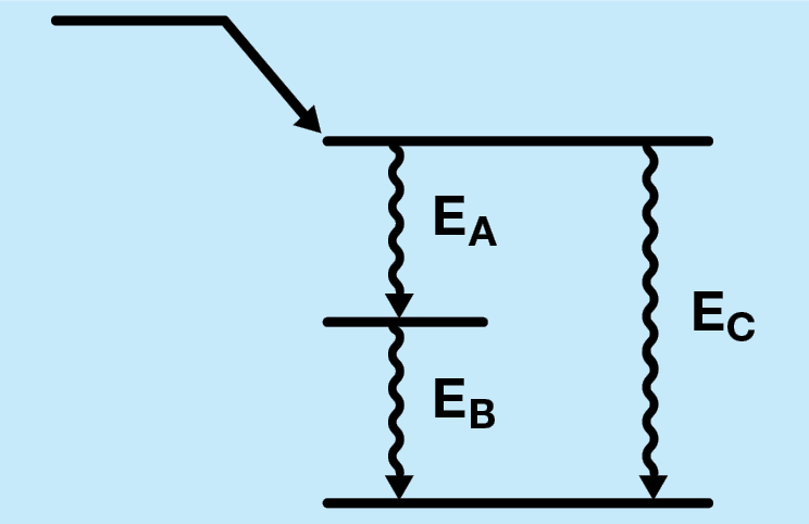
Figure 12-3: Decay schema demonstrating “summing in” effect for energy EC.
The typical lifetime of excited states in a nucleus is in the picosecond time scale. The typical response time for a detector, i.e., the minimum time between two photon events that is needed for the detector to recognize these as two separate events, is in the order of microseconds. Note that this is several orders of magnitude longer than the typical lifetime of the excited states. For decays where more than one photon is emitted there is a significant probability that multiple photons will interact with and deposit energy in the detector. Since the time between the photon emissions is much shorter than the response time for the detector, it is not possible for the detector to distinguish the photons as separate events and only one pulse is generated, which corresponds to the sum of the individual deposited energies. Figure 12-2 shows an example of a decay emitting two photons with both photons depositing energy in the detector within the detector’s resolving time. This event is called true-coincidence summing, or cascade summing. Two cases require special attention:
1. Summing Out In this event, one of the photons deposits all of its energy in the detector (for example the 1173 keV gamma ray in Fig 12-1) and the other photon (for example the 1332 keV gamma ray) deposits some or all of its energy in the detector. This will move a count from the full-energy peak of the first photon (at 1173 keV for this example) to a higher energy in the spectrum. This reduces the count rate of the first photon compared to the detection of only a single photon. This phenomenon is called summing out.
2. Summing In This effect is relevant when the gamma energy of interest is equal to the sum of the energy of two other gamma rays in the decay schema like the example in Fig 12-3. Here summing between gamma rays of energy EA and EB will cause an increase in the count rate of the peak at energy EC. This is called summing in.
Gamma-X-ray coincidence
There are two ways that X-rays can be produced so that they will contribute to true-coincidence summing.
1. Electron Capture Here one of the closely-bound electrons is captured, creating a vacancy on one of the inner electron shells. Electrons from the outer shells will fill the inner-shell vacancy and emit X-rays that can be detected. Since these X-rays are created from the initial decay, every photon emitted from the daughter nucleus can be detected in coincidence with the X-rays (including cases where a single photon is emitted). This is an example of summing out.
2. Internal Conversion Internal conversion is a process when the excited nucleus interacts with the electron cloud around the nucleus and the excess energy is transferred to one of the electrons which will be emitted from the atom. This will create a vacancy in one of the electron shells which will be filled by an outer electron and an X-ray will be emitted, similar to electron capture described above. This is also an example of summing out.
Gamma-annihilation photon coincidence
There are cases where photons created by the decay process (such as in β+ decay) can sum with the photons from the daughter nuclide. In β+ decay, positrons are emitted which will slow down in the surrounding material, find an electron and annihilate emitting two back-to-back photons with an energy of 511 keV. The time it takes for the positron to slow down and annihilate is short compared to the response time of the detector. If at least one of the photons from the annihilation deposits energy in the detector in addition to detection of a photon in the daughter nucleus then the count will be moved from the full energy peak. This is another case of summing out as described above.
Probability of true-coincidence summing
Because true-coincidence summing requires the detection of two photons from the same decay it is strongly dependent on the following:
1. The detection efficiency for the photons that participate in the summing process. This is a function of the detector type and the counting geometry that is used. For example, the probability of detecting two photons as a summed event increases with increasing detector size and decreasing source-to-detector distance.
2. The nuclide that is being measured. More specifically, the decay schema of the nuclide. Earlier we have learned that summing in and out depends on the gamma-ray decay schema (e.g. the presence of a cascade and the mode of decay, such as internal conversion or electron capture). There are some nuclei that are unaffected (such as 137Cs) and others (such as 60Co and 88Y) that demonstrate significant summing effects.
Consequences for source-based efficiency calibrations
Most commercially available multi-gamma sources include nuclides that exhibit true-coincidence summing. For example it is common to use 60Co and 88Y as the high-energy photon-emitting nuclides and both of these suffer from summing out. Using nuclides that have summing-out effects in close geometries will result in peak count rates that are lower than they would have been if the nuclide didn’t have summing-out effects. The result of this is that the efficiency at these energies will appear to be lower than the true efficiency. If these efficiency points are used without correction, then the calculated efficiency will be biased low compared to the true efficiency. As a result, when the efficiency is used to calculate the activity for a summing-free sample measurement the result will be higher than the true activity.
Consequences for sample counts
For sample counts, the summing-out effects will cause a reduction in the measured peak count rates; the measured activities will therefore be lower than the true activities. Summing in has the opposite effect, with measured activities exceeding the true activities. It should be noted that summing-out effects are most common. It is also the more significant effect since the underestimating of nuclide activities can have safety implications.
Reducing the effect of true-coincidence summing
Since the probability of true-coincidence summing is dependent on the detection efficiency, the effect can be reduced by moving the sample away from the detector. However, the impact of reducing the overall efficiency of the counting system can result in increased counting times (in order to maintain counting statistics) and therefore reduced productivity for sample counting.
If the coincidence summing is mainly due to X-rays (as may be the case when the nucleus decays by electron capture) then the coincidence summing can be reduced by introducing an attenuator that will attenuate most low energy photons. The optimum treatment is to use software, such as LabSOCS calculations, to quantify and correct for true-coincidence-summing effects. This approach is applicable for all measurement geometries and all commonly measured nuclides that are known to be affected.
Experiment 12 Guide:
Measurements
1. Ensure that the Lynx II DSA (with the HPGe detector connected) is connected to the measurement PC either directly or via your local network.
2. Place the 137Cs source in front of the detector.
3. Open the ProSpect Gamma Spectroscopy Software and connect to the Lynx II DSA.
4. Configure the MCA settings as recommended in Experiment 7.
5. Use the software to apply the recommended detector bias to the HPGe detector.
6. Set the PHA conversion gain to 32768 channels
7. Set the amplifier gain such that the full-energy peak is close to 40% of the spectrum.
8. Make an energy calibration.
9. Position the 137Cs source on the endcap and acquire a spectrum (use a count time such that there is at least 10 000 counts in the full-energy peak).
10. Make a record of the number of counts in the full-energy peak(s).
11. Position the 137Cs source 5 cm from the source and acquire a spectrum (use a count time such that there is at least 10 000 counts in the full-energy peak).
12. Make a record of the number of counts in the full-energy peak(s).
13. Position the 137Cs source 30 cm from the source and acquire a spectrum (use a count time such that there is at least 10 000 counts in the full-energy peak).
14. Make a record of the number of counts in the full-energy peak(s).
15. Position the 137Cs source on a thin copper sheet directly on the endcap and acquire a spectrum (use a count time such that there is at least 10 000 counts in the full-energy peak).
16. Make a record of the number of counts in the full-energy peak(s).
17. Repeat step 16 for a 60Co source.
18. Repeat step 16 for a 22Na source.
19. Repeat step 16 for a 152Eu source.
Analysis
1. In LabSOCS Geometry Composer create a model of the point source at the three different distances and with the copper absorber. Calculate the efficiencies for all the energies for which peak areas were calculated.
2. Using the peak areas, count times and the known photon-emission rate for the sources (it can be found on the source certificate) calculate the efficiencies for all sources and geometries.
3. Calculate the true-coincidence-summing factor (defined as the measured efficiency divided by the calculated efficiency) for all sources and geometries. A factor close to 1 indicates that there is no or negligible true-coincidence summing. A factor less than 1 indicates that there are summing-out coincidences and a factor larger than 1 indicates that there are summing-in coincidences.
4. For each source and geometry explain the value of the true-coincidence-summing factor. If necessary look up the decay scheme from a book or online, for example from the National Nuclear Data Center at Brookhaven National Laboratory http://www.nndc.bnl.gov/nudat2/.