Technical Advantages of ISOCS / LabSOCS

December 6th, 2022

Introduction

The advantages of mathematical calibration software are now well understood across the nuclear measurement industry. The elimination of traditional calibration sources provides significant savings in cost and measurement time. In addition, the flexibility of these tools allow excellent replication of the measured sample geometry resulting in improved accuracy over fabricated calibration source standards.

There are now several mathematical calibration software packages in use by laboratories and nuclear facilities. This application note provides a technical review of the Mirion ISOCS / LabSOCS software for some typical application scenarios in order to provide some quantitative evidence of its advantages over the alternatives. The focus is on several aspects of the mathematical calibration that have a significant impact on the accuracy of the measurement result.

Intrinsic Detector Efficiency

ISOCS / LabSOCS software differ from the other available mathematical calibration packages in that a full factory characterization is performed on the detector. This process uses NIST-traceable sources and the well-known MCNP ^® Monte Carlo modeling code. The radiation response profile of each individual detector in free space is determined for a 1000 meter diameter sphere around the detector covering an energy range of 10 keV through to 7 MeV. In the software, the characterized detector is selected from a list of available detectors – it then becomes incorporated into the model. At this point, the user need only worry about the sample geometry (i.e. the location and physical properties of the item being measured and the location and distribution of the source). The software does not require any additional information relating to the detector itself, this information is automatically extracted from a detector characterization file that is generated through the characterization process and is shipped with the detector on CD.

This method contrasts those used by alternative solutions, which actively promote the fact that a factory characterization is not required. These alternative methods have significant drawbacks driven by need for accurate detector crystal dimensional information. This information is entered into the modeling software packages in order to determine the intrinsic detection efficiency. The issue is that it is not possible to precisely know the details of the actual detector crystal inside the can (for example the actual shape, the active volume around corners and edges, the dead-layer thickness, the amount of bevel and the position of the cold detector in the can). Differences between the intrinsic detection efficiency calculated from the manufacturer’s dimensional information and the actual intrinsic detection efficiency can cause significant measurement bias. ISOCS / LabSOCS software eliminates this bias since the actual detector crystal is accurately characterized.

In order to quantify a typical level of bias associated with assumed detector dimensions, some LabSOCS detector efficiency curves have been generated for a typical detector type, a 44% SEGe detector. The dimensions of the detector crystal were varied to an extent that is typical of detector manufacturing tolerances. Figure 1 below illustrates the uncertainty envelope for the efficiency, based on the typical dimensions and uncertainties for the crystal listed in the figure.

Figure 1:
Uncertainty envelope associated with the variable detector dimensions shown at the top of the figure

These data illustrate that these typical manufacturing uncertainties cause a ±8 – 10% uncertainty in the detector efficiency response at mid-range (100 – 400 keV) to high energies. For energies less than 100 keV these deviations can be even worse (around ±15% for the Am-241 60 keV emission energy). Also note that the variances in the above figure do not include other parameters that affect the detector efficiency such as the germanium well depth and diameter and the crystal bevel.

It should be noted that in addition to HPGe detectors, ISOCS/ LabSOCS software has also been successfully applied to both LaBr3 and NaI detectors.

Modeling the Sample Geometry

Once a characterized detector is selected in the ISOCS / LabSOCS software, the user can focus solely on generating an accurate model of the sample geometry (and no longer needs to be concerned with the detector itself). Differences between the modeled geometry and the actual geometry are a significant source of measurement bias associated with this part of the process. The important sources of bias include:

Location of the sample relative to the detector
Distribution of the source within the sample
Physical properties of the sample (e.g. shape and thickness of container, density of the source matrix, material composition of the container and matrix)

The ISOCS / LabSOCS solution has five key benefits relating to sample geometry definition:

A broad range of validated geometry templates – minimizing the extent of geometry modifications
The high degree of flexibility required to accurately simulate the physical characteristics of the sample
The Line Activity Correlation Evaluator (LACE) tool allowing validation of the assumed sample characteristics, thus helping to remove measurement bias
The ISOCS Uncertainty Estimator tool allowing robust treatment of total measurement uncertainty where physical sample characteristics are poorly known. It also facilitates a sensitivity analysis to highlight the most critical characteristics for your measurement
Run-time queries allowing the entry of key information about the sample during the analysis. The efficiency calibration is automatically computed as a part of the sample assay.

Each of these five benefits is described in detail below.

Broad Range of Geometry Templates

We supply a versatile set of qualified geometry templates with both LabSOCS and ISOCS software. The LabSOCS templates are designed to be applicable to laboratory counting, while the ISOCS templates cater for in situ applications.

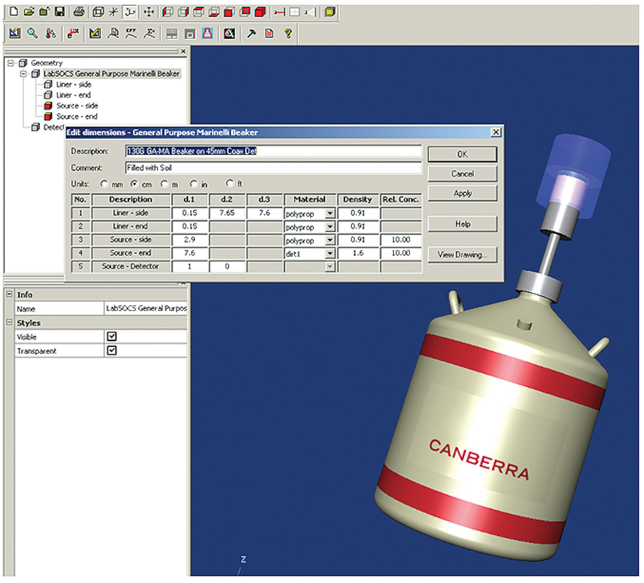
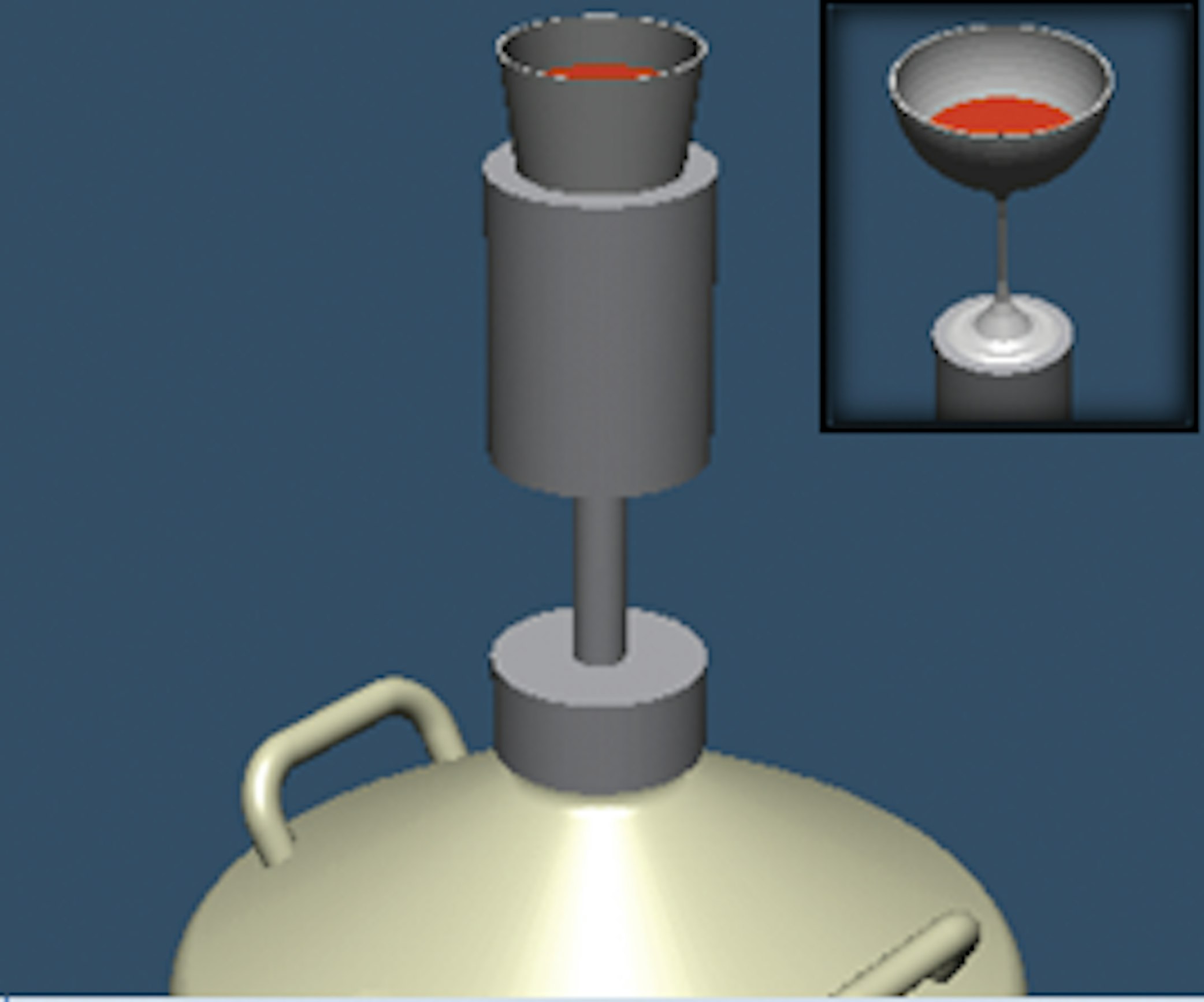
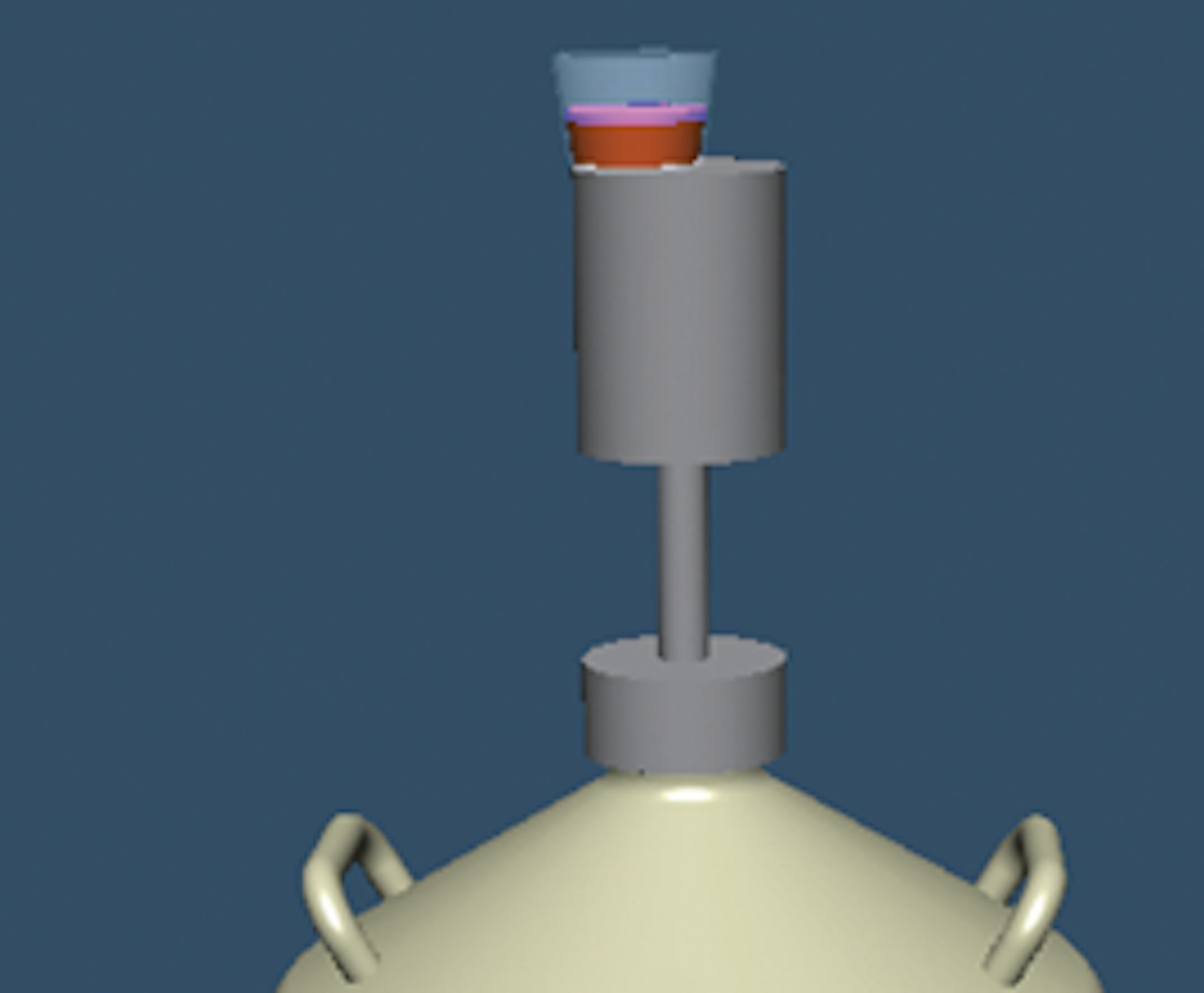
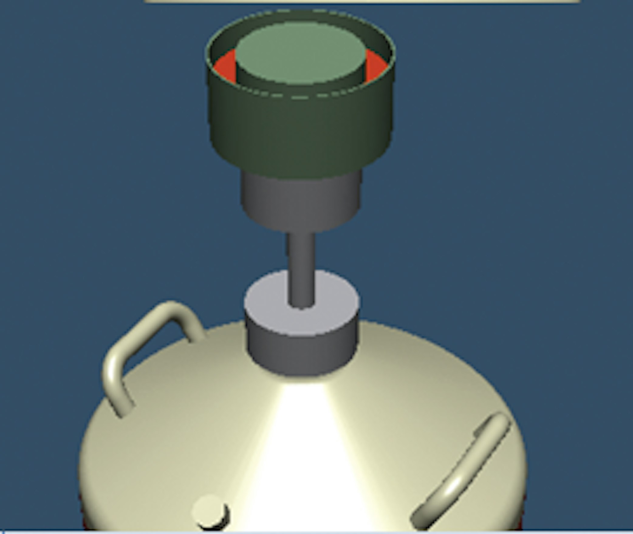
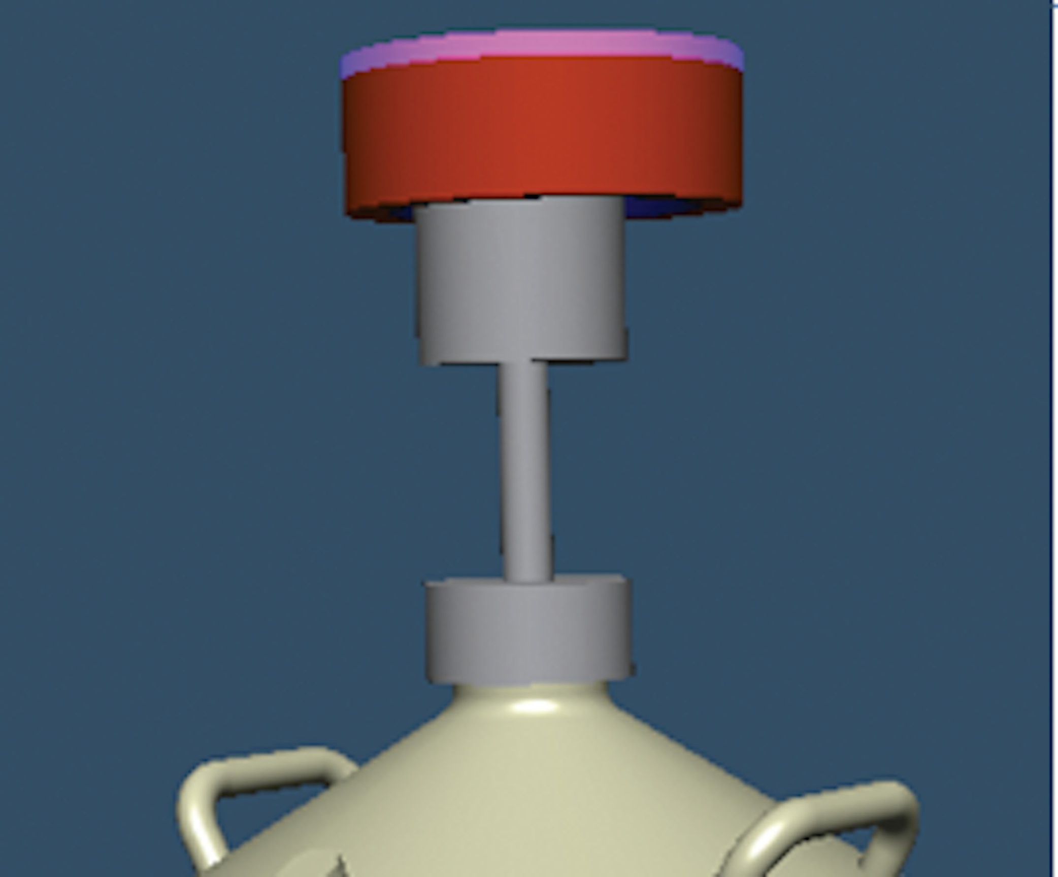
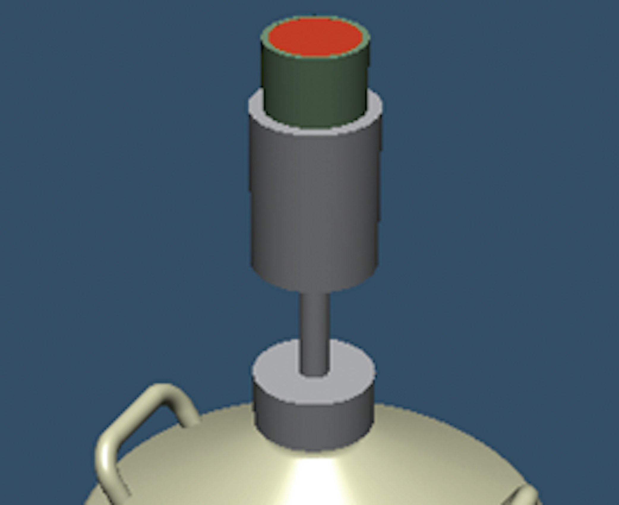
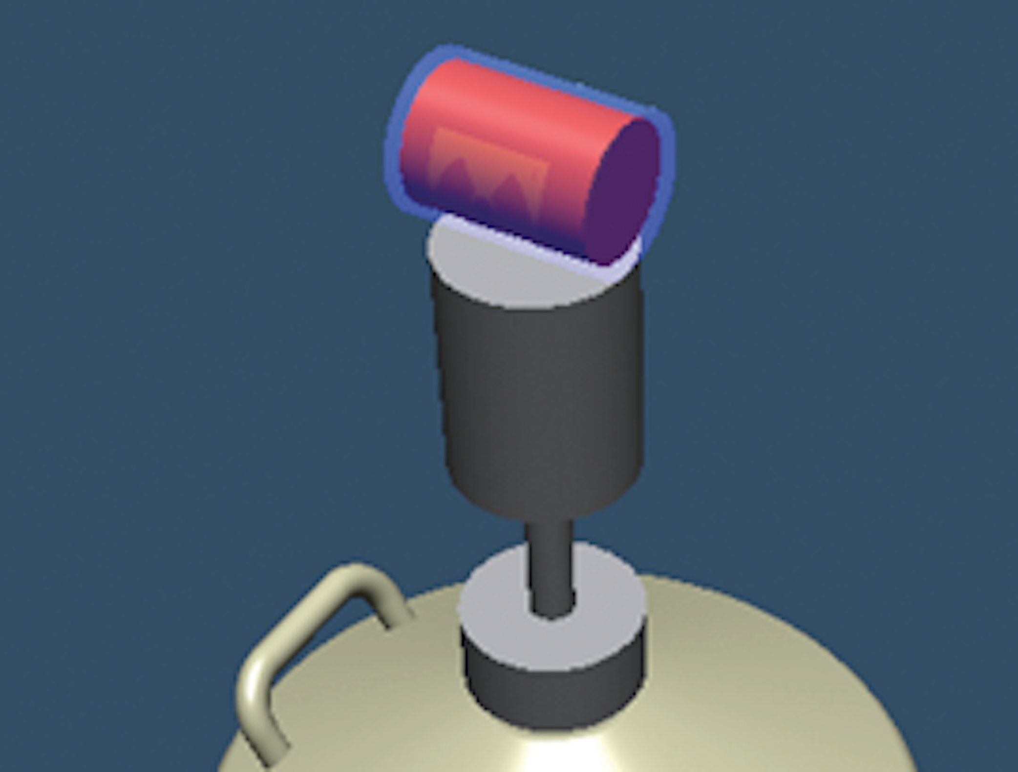
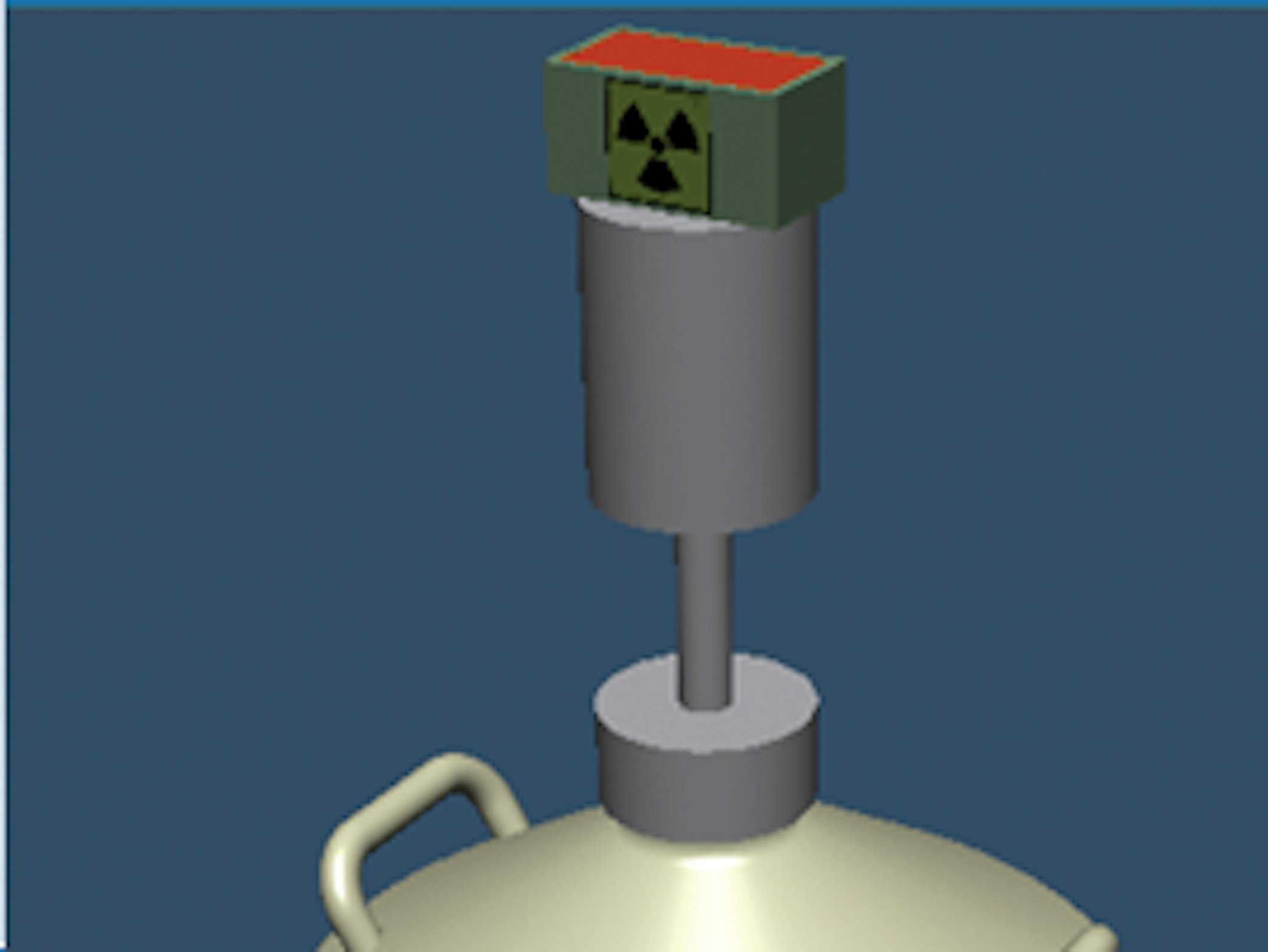
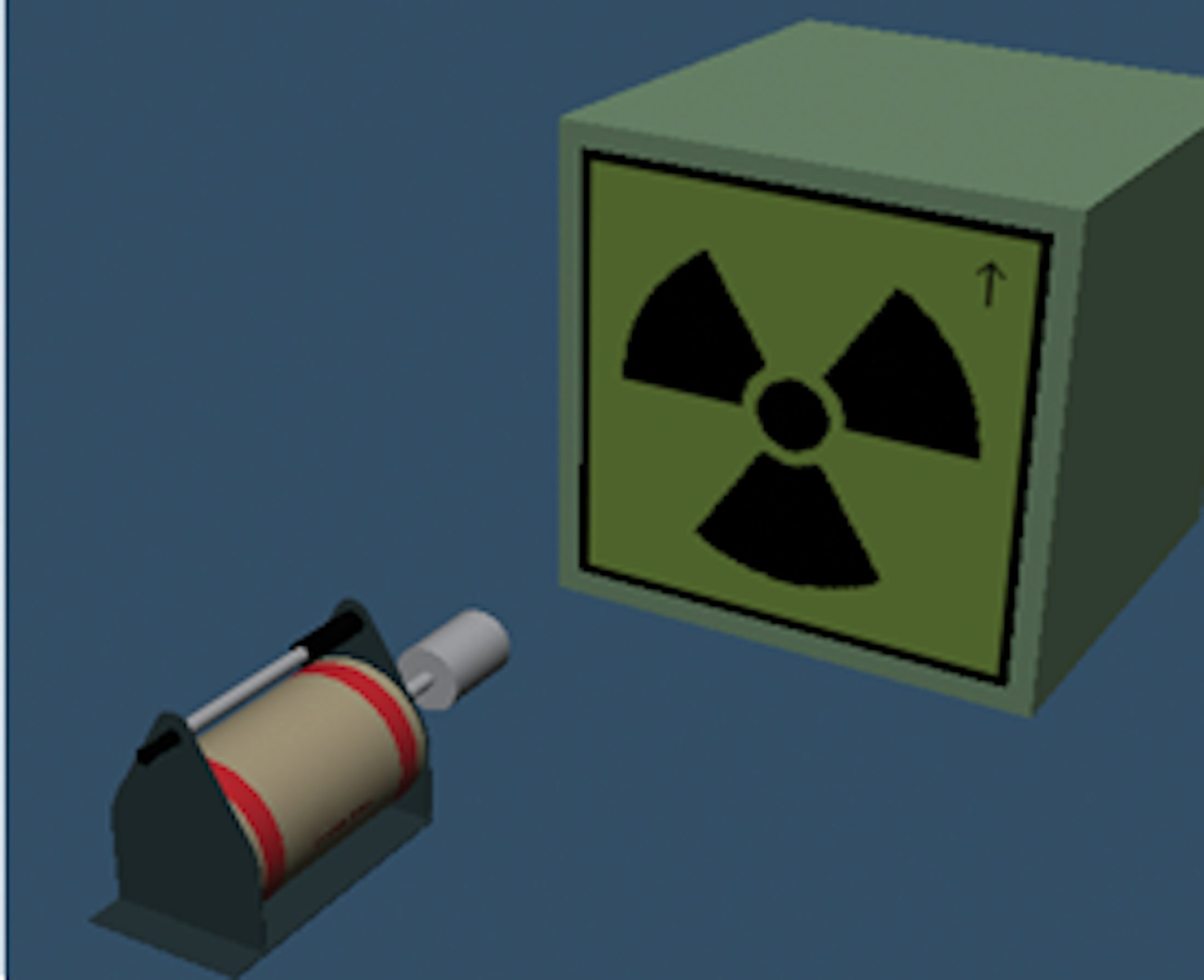
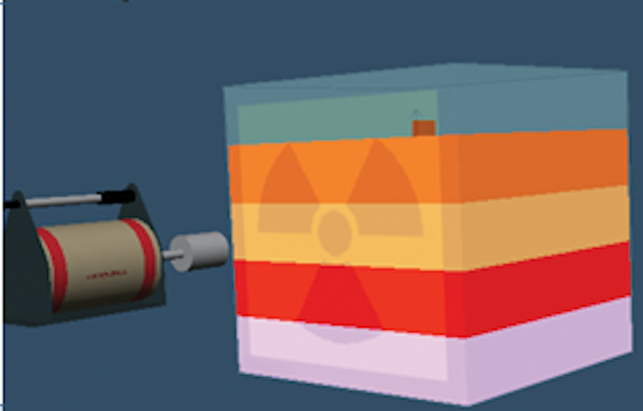
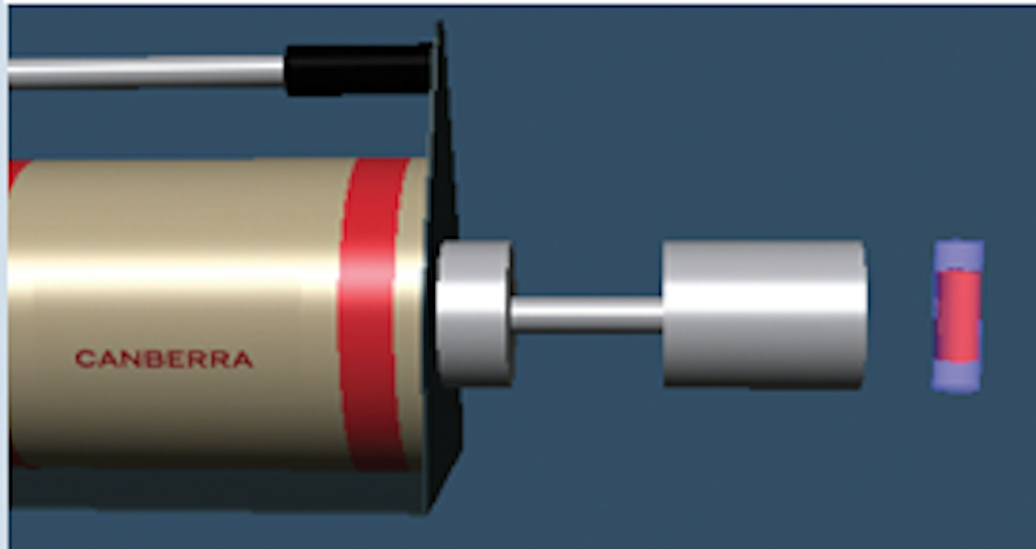
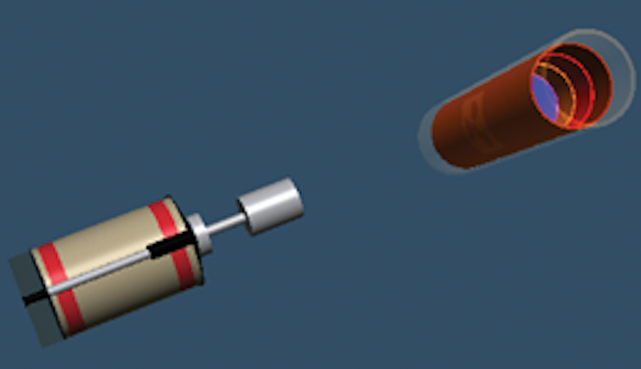
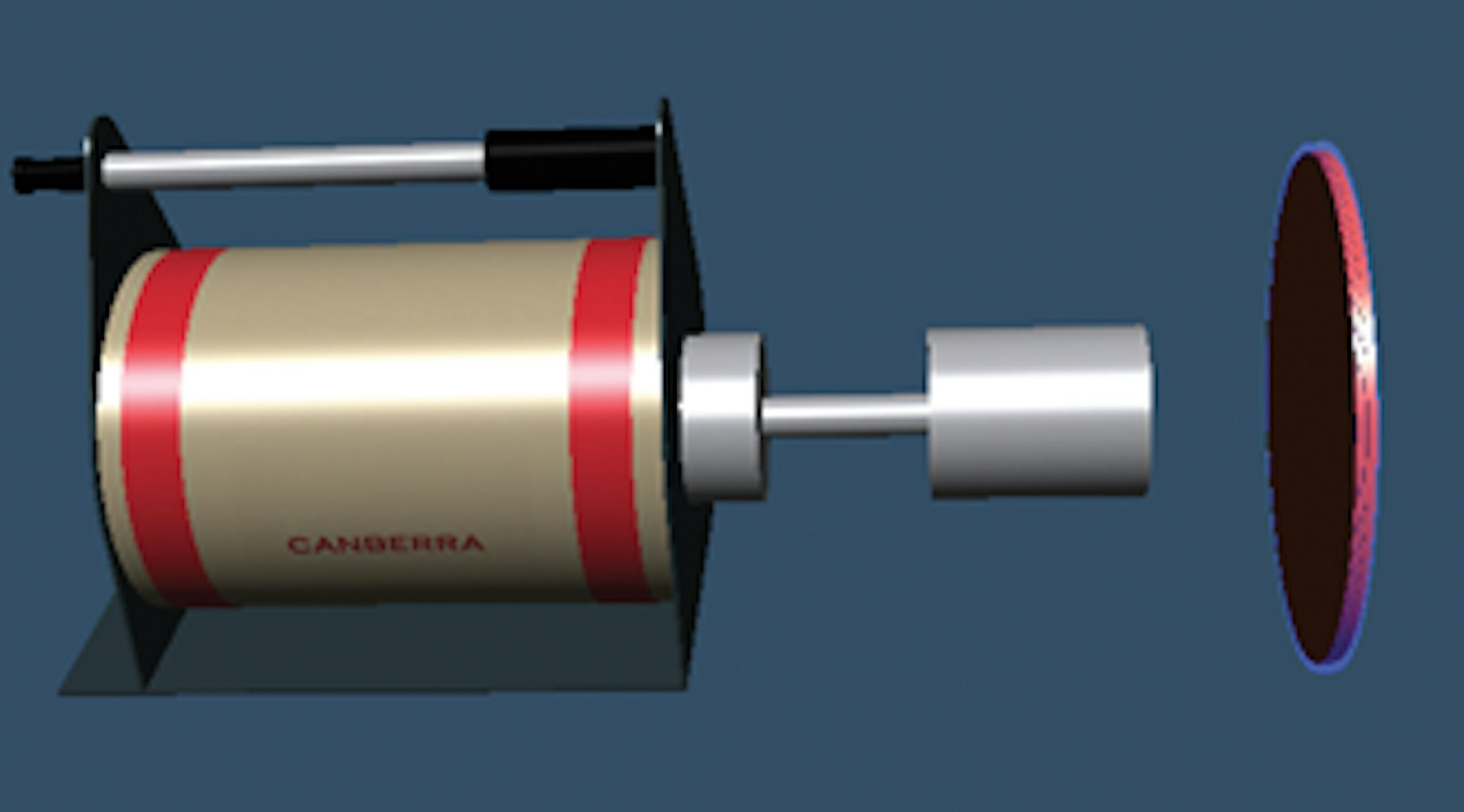
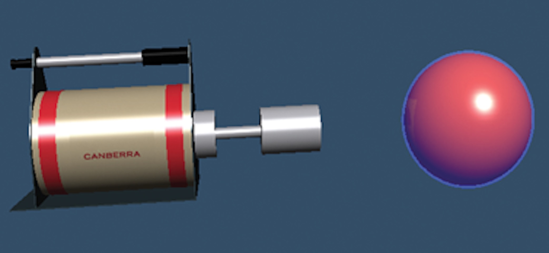
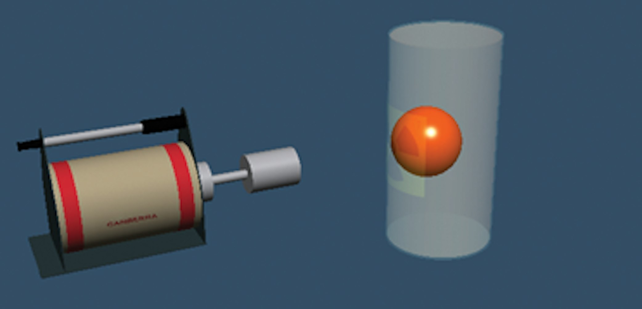
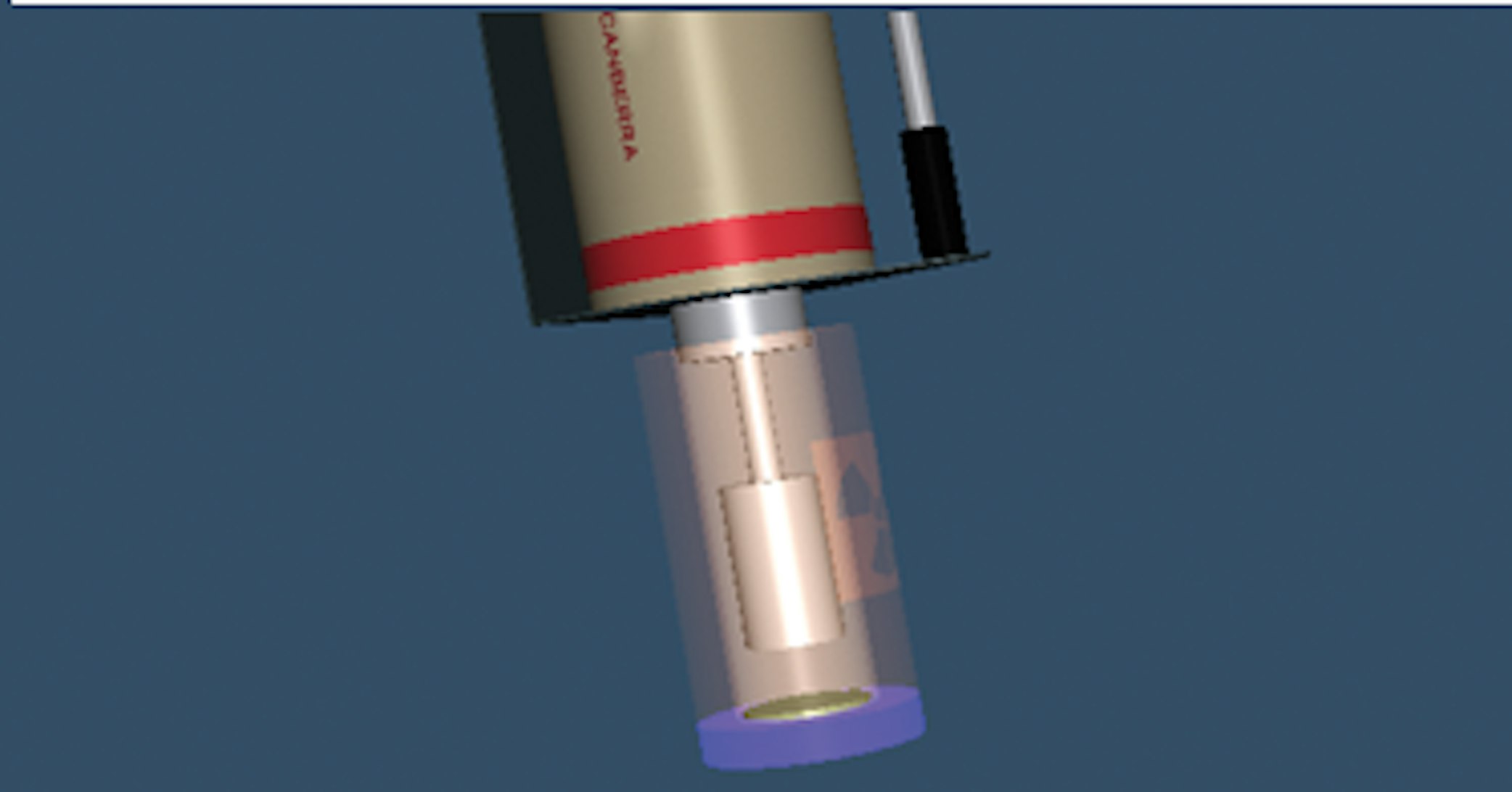
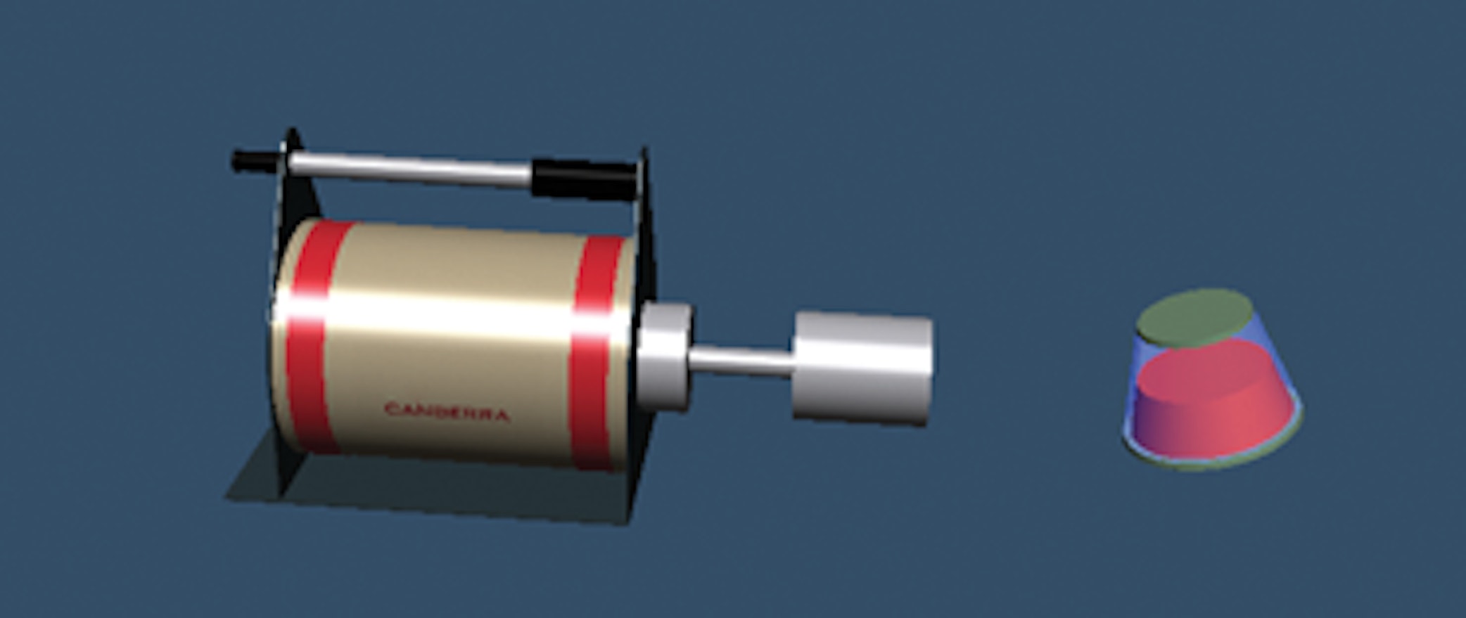
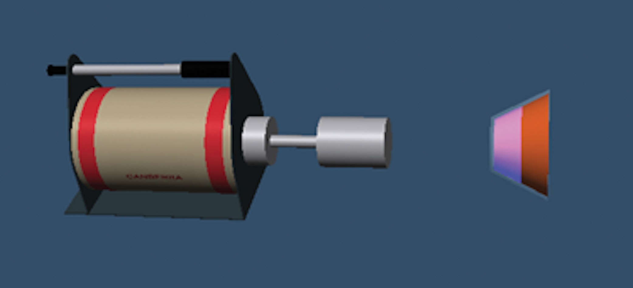
The purpose of these templates is to minimize the amount of geometry modeling that must be done by the operator. The operator makes a few simple physical measurements of the sample (e.g. the location of the sample relative to the detector, the dimensions of the sample container and the sample density) and these are input through the intuitive 3D Geometry Composer interface (see Figure 2). This provides visual feedback through the 3D interface that the model has been correctly generated (this is facilitated through point of view rotation, options for transparency and other field of view options).

Figure 2:
3D Geometry Composer for model generation

LabSOCS Templates

Simplified Beaker

Used for rotationally symmetric laboratory containers of any shape (such as glass beakers, filter papers charcoal canisters, etc.). Either simple cylindrical or conical containers can be defined.

Complex rotationally symmetric containers can be custom-generated by the users with the Beaker Editor application (an example – a wine glass- is shown as an insert).

General Purpose Beaker

For special cases for simple beakers where:

There are multiple sample layers
The axis of the sample container does not coincide with the detector axis

The Beaker Editor can also be used for custom models.

Simplified Marinelli Beaker

Used where the container is a Marinelli Beaker.

General Purpose Marinelli Beaker

For special cases for Marinelli Beakers where:

a) There are multiple sample layers

b) The axis of the sample container does not coincide with the detector axis

Cylinder

Where the sample is a simple cylinder (e.g. pipes).

Cylinder from the side

A basic bottle or other cylinder (assumed to be full) viewed from the side.

Simplified Box

A basic rectangular carton or box, viewed from the base of the box.

Simplified Sphere

Where the sample is a simple sphere.

Disk

Where the sample is a disk (e.g. an air filter).

Point

For modeling weightless point sources.

ISOCS Templates

Simple Cylinder

A basic barrel, tank or drum.

Complex Cylinder

Like the simple cylinder, but allows the contamination to be distributed in up to four different layers and placement of an additional concentrated source anywhere inside the container.

Simple Box

A basic rectangular carton or waste shipping container. This can also be used to simulate a truck filled with scrap material or a small building.

Complex Box

Like the simple box, but allows the contamination to be distributed in up to four different layers and placement of an additional concentrated source anywhere inside the container.

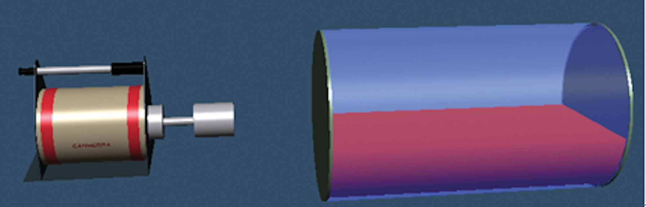
Pipe

A pipe (empty or full) that can contain material that has plated out or built up on the inner wall surface.

Complex Pipe

Like a pipe, but allows multiple layers of contamination layers and placement of an additional concentrated source anywhere inside the container.

Rectangular Plane

Typically used for floors, walls or ceilings and commonly used for soil measurements. The source can be defined on the surface or behind up to 10 layers of absorber (e.g. paint, paneling, floor coverings, etc.).

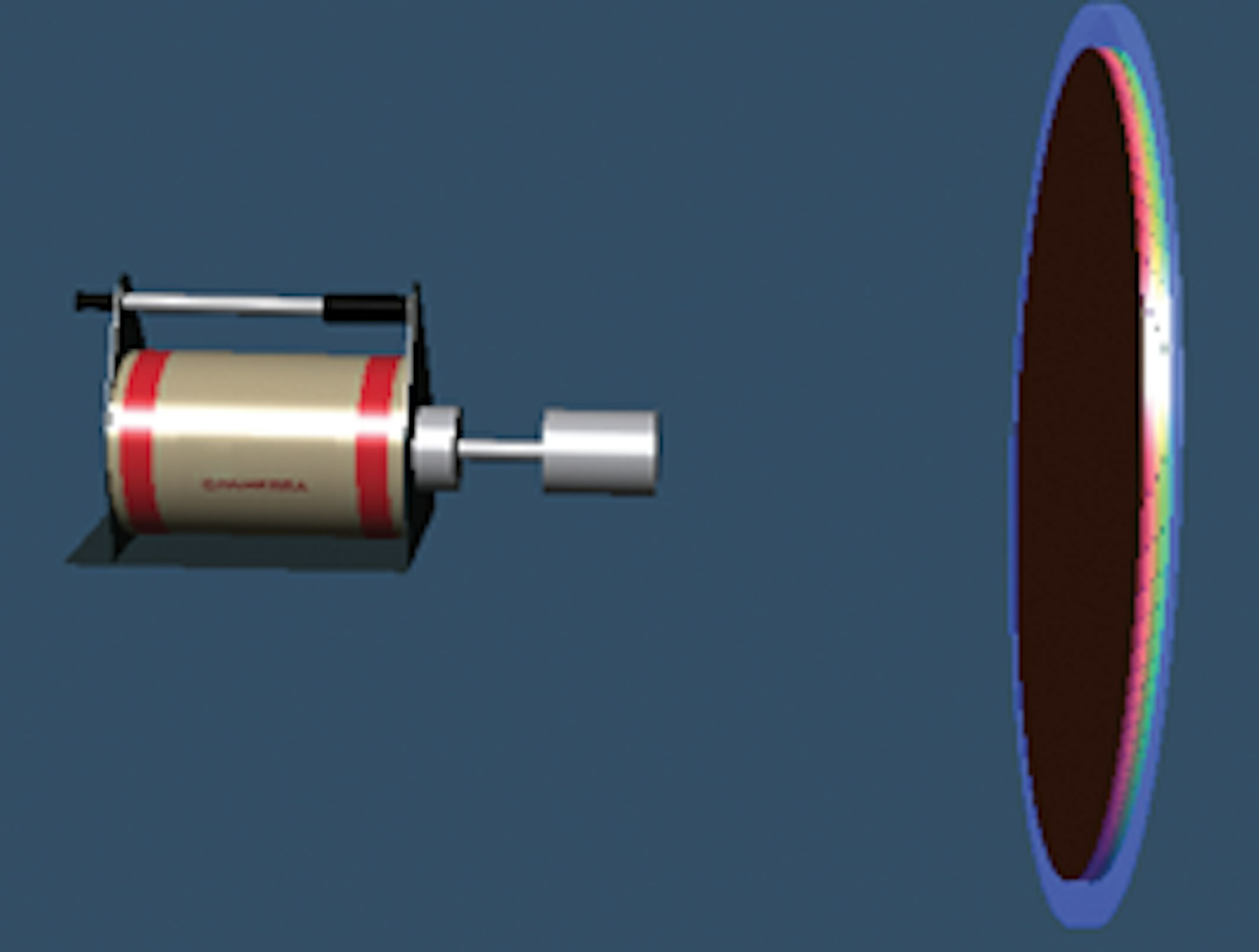
Circular Plane

Typically used to measure the end of a barrel, drum or tank and commonly used for soil measurements. As with the rectangular plane, allows specification of up to 10 layers of absorption.

Tank

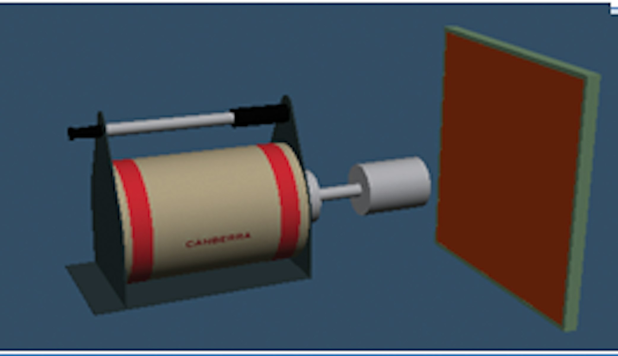
A full or partially filled horizontal cylindrical container, such as a tank or drum lying on its side. It can be viewed from the side or end.

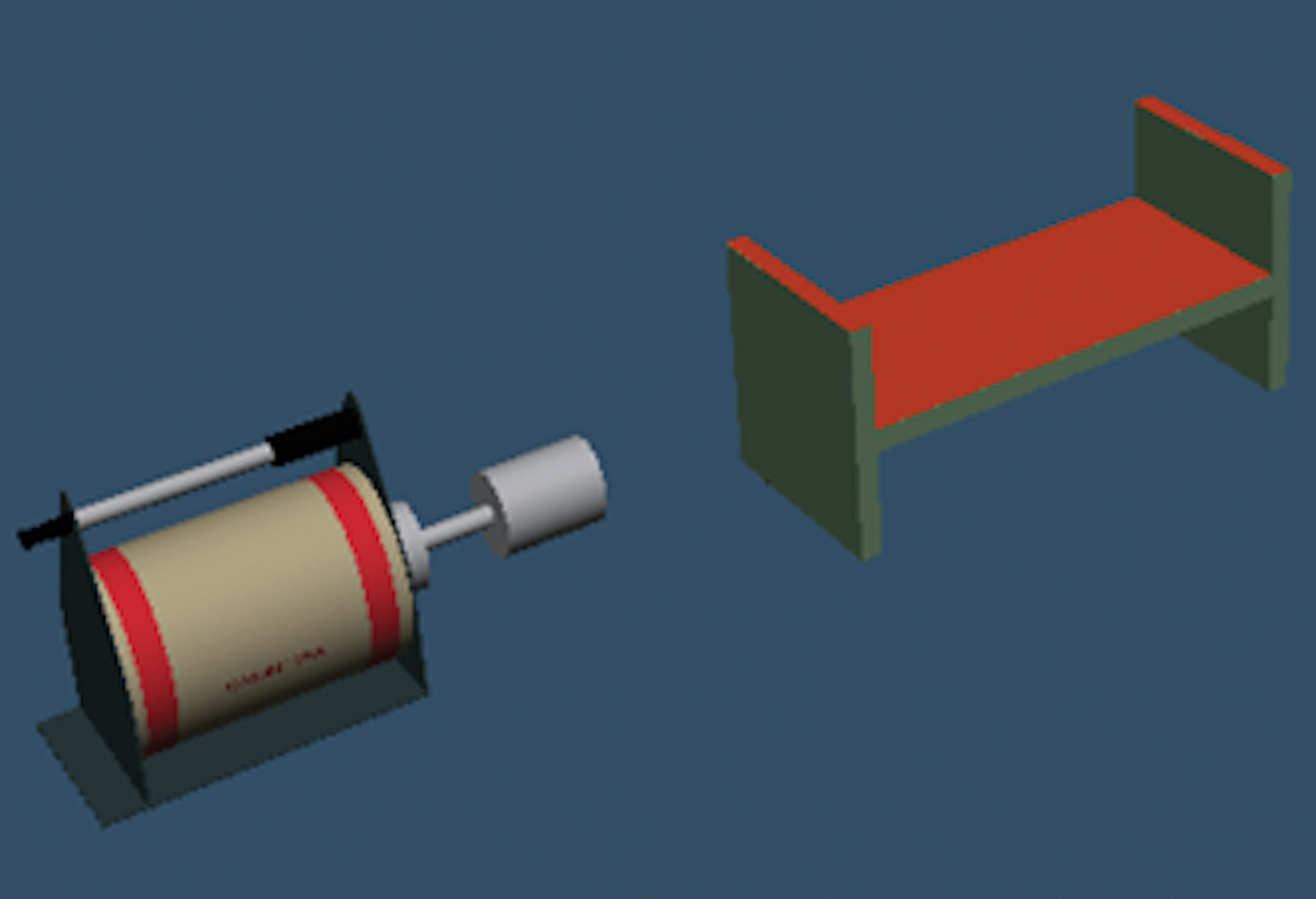
Surface Contamination Templates

This is a series of templates that allow thin layers of surface contamination to be measured in specified locations on variously shaped objects. These include:

H or I beams (as shown in example)
L angles or beams
Pipes or tubes
C or U channels
Room walls, ceilings or floors
Regular tubes or boxes

Exponential Circular Plane

Like the circular plane, but this can be used to model a realistic depth distribution of activity. This can either be a simple decreasing exponential distribution or activity with an initial build-up followed by a simple exponential decrease.

Sphere

For internally contaminated spherical objects such as large pipe valves.

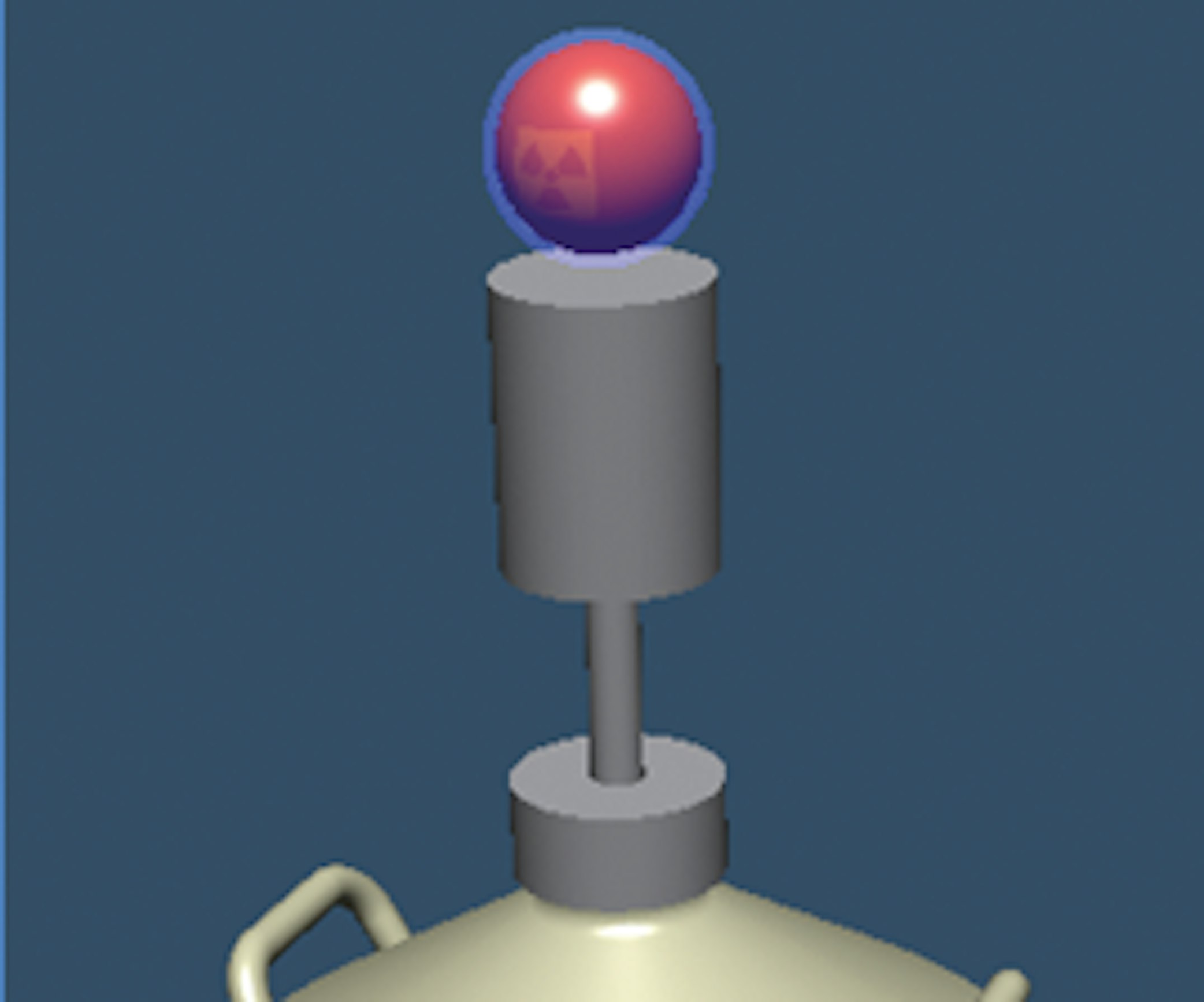
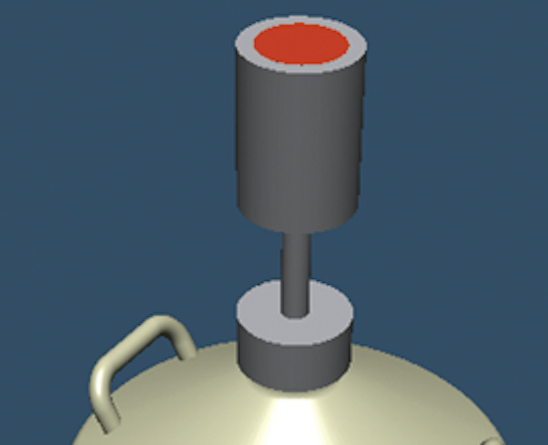
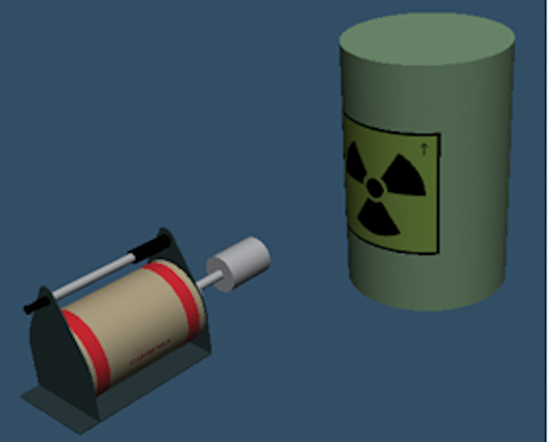
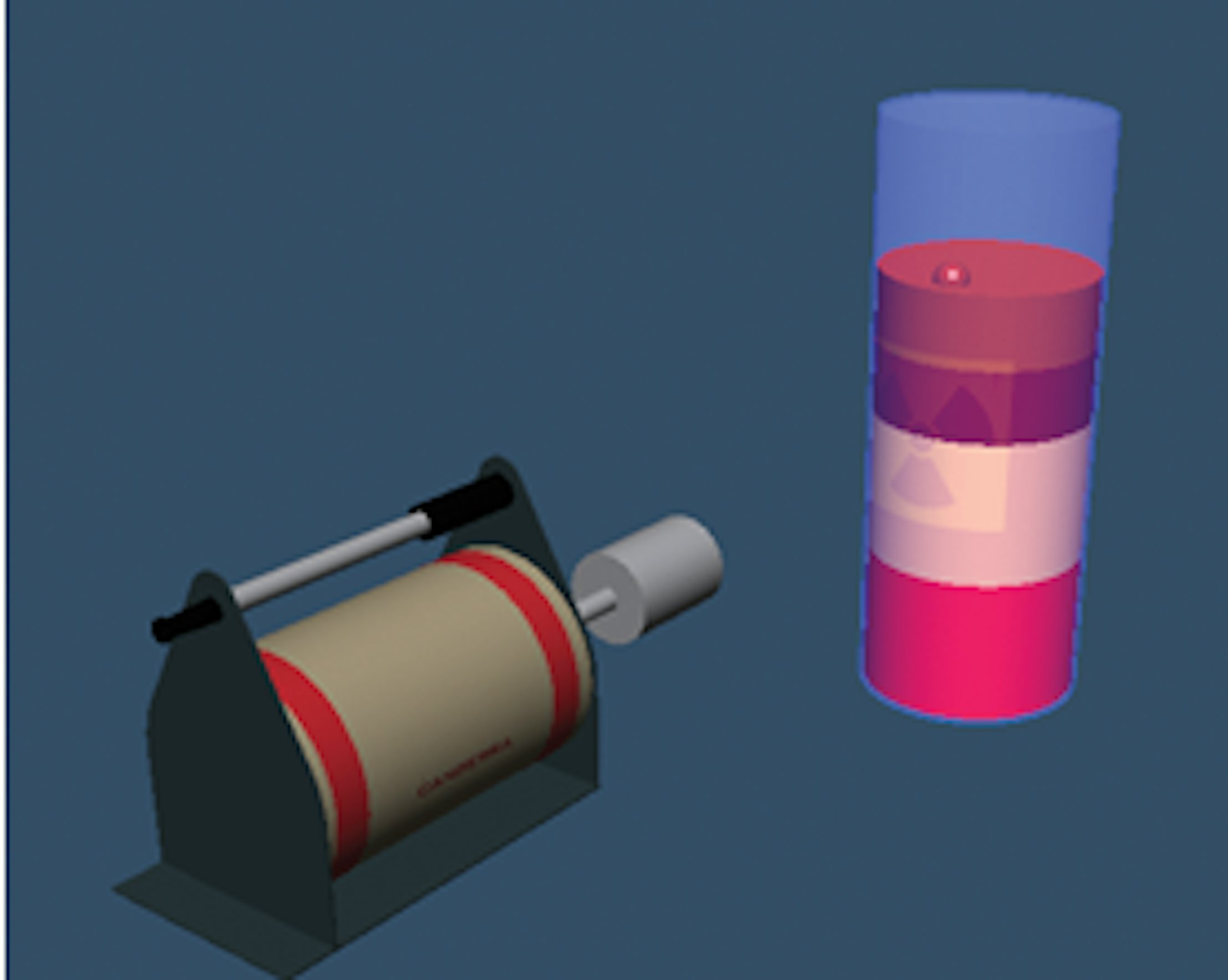
Special Sphere

A spherical sample located inside a vertical cylindrical container (such as a drum) viewed from the side. The source can be defined with up to seven spherical layers.

Well or Marinelli Beaker

For modeling subsurface soil in well logging, or standard Marinelli Beaker sample containers.

Cone Viewed from the Side

A vertical conical container viewed from its side, such as a tapered tank or a pile of sand or soil with sloping sides.

Cone Viewed from the Bottom

Like the cone template but the detector viewing the bottom of the cone.

The supplied templates closely replicate the shapes and source distributions for a range of common sample counting geometries. These are designed to minimize the amount of data entry required to construct the model of the sample, since this is a potential source of error. Since the templates are benchmarked and tested prior to release, the small amount of modification required leads to a high degree of confidence in the robustness of the model, and therefore of the results.

Other efficiency calibration software packages offer simple shapes only (e.g. cylinder, spheres, disks) with a high degree of modification required (and therefore significant user intervention) to generate a shape that approaches the actual counting geometry. In these cases the model may be a compromised approximation of the sample. This can lead to measurement bias, as discussed in more detail in the section below.

Flexibility in Constructing the Container Shape

The templates presented above demonstrate the flexibility of the software to accurately describe the actual shape of the measurement container (e.g. curved walls and concave bases). Many other modeling packages do not allow these curvatures to be accounted for, and such compromises can cause significant measurement bias. This is particularly important for close counting, for example environmental monitoring applications where sample is placed directly on the detector end cap.

To demonstrate this, an efficiency calibration curve was generated using LabSOCS software for a typical beaker positioned on the end cap of a BE5030 detector. The assumed application was drinking water analysis with a volume source in a 400 ml water matrix. The beaker has a concave base giving a maximum gap of 6 mm between the base of the beaker and the detector end cap (as shown in Figure 3 below).

Figure 3:
Environmental Monitoring Scenario

Several other efficiency calibration software packages are unable to simulate curved container walls, and in this respect LabSOCS software offers significant advantages over the alternatives. In order to quantify this, the example in Figure 3 was used to determine the level of bias associated with assuming a flat bottomed beaker. To determine this, an efficiency calibration curve was also generated assuming a flat beaker base (with no gap between the beaker and the detector end cap).

The results are presented in Table 1.

Table 1 demonstrates that the compromise in the accuracy of the model (due to limitations in constructing curved surfaces) can result in a bias in the measured efficiency calibration of +6% for this typical application. This assumes that the beaker is filled to near capacity. If the beaker is only partially filled, the observed bias can be as high as +15%. A high positive bias in the efficiency model can lead to an under reporting of the nuclide activity by the same magnitude.

This study provides indicative information on the expected bias for only one typical application. Other similar sources of bias include rounded corners of containers, tapered containers, and other objects such as centering rings, mounting platforms, and x-ray filters. All of these objects can be readily modeled in ISOCS/LabSOCS software.

Nuclide (Energy)	Efficiency (concave base)	Efficiency (flat base)	Efficiency Ratio (concave/flat)
Am-241 (60 keV)	0.00531	0.00553	1.04
Cs-137 (662 keV)	0.00141	0.00149	1.06
Co-60 (1332 keV)	0.000816	0.000864	1.06

Checking the Physical Properties

Sometimes in a sample measurement it is not possible to accurately measure one or more of the physical characteristics of the sample (for example the material composition or density of the sample matrix or of any absorbers present). The Genie™ 2000 software package includes a very useful tool, the Line Activity Consistency Evaluator (LACE) that can be used to determine the optimum values for unknown parameters.

LACE exploits one of the fundamental rules of quantitative gamma spectroscopy, that all lines within a nuclide must have the same activity. After the nuclide activity results have been calculated, LACE plots the activities as a function of the line energy. These results are normalized to either the mean activity or a key line activity. The gradient of the resulting graph should be close to zero, since the activity should be independent of line energy. The gradient can provide useful information that can be fed back into the model in order to improve the accuracy of the efficiency calibration. Note that outlier data points can indicate interference or other peak fitting issues.

Figure 4 shows three LACE plots that represent three different measurements. Each measurement used a LabSOCS model with a different assumed sample matrix density (0.575, 1.15 and 2.3 g/cm³). In this case, the optimum density is 1.15 g/cm³. Positive gradients indicate that the assumed sample matrix density is too low. Conversely, negative gradients indicate a high assumed density. Selecting the optimum values for the sample’s physical characteristics removes measurement bias at the level of 5–10%.

The ISOCS Uncertainty Estimator (IUE)

This is a powerful application that allows the user to investigate the impact of probabilistic variation one or more of the physical parameters of a geometry. Previously this was done by generating multiple models with the physical parameters set to different values; the IUE offers a quicker and easier automated method. The IUE allows variation of the input parameter(s) within a defined range. The tool simultaneously varies these parameters (through iteratively creating and analyzing multiple models based on the standard input model).

For example consider a drum partially filled with waste material. The exact fill height is not known, but you are able to bound this parameter (for example based on measured drum mass and volume). IUE allows you to determine the range of total activity based on the range in fill height. IUE facilitates automated calibrations of multi-detector, scanning and rotating sample geometries. It also allows simulation of multiple hotspots with random size and locations within the container in order to study the effect of uncertainties in the source distribution.

The IUE can be operated in two modes:

To estimate Total Measurement Uncertainty (TMU) – to generate a mean efficiency calibration with uncertainties at each calibration point. This provides a robust TMU where one or more of the physical sample parameters are not well known or are variable.
To perform Sensitivity Analyses – in this mode IUE is an excellent measurement planning tool. It allows the user to easily determine the impact of systematic error in the sample geometry model on the TMU.

Figure 4:
LACE Results for three different assumed matrix efficiencies for measurement of Eu-152.
The line activity is normalized to the key line activity, in this case the 344 keV line.

ISOCS/LabSOCS Efficiency Corrections at Run Time

The gamma spectroscopy software offers an extremely useful tool which provides flexibility in how laboratories operate. Traditionally, it has been necessary to generate a limited set of calibrations in advance of sample measurements. Expensive and time-consuming sample preparation time is then spent in order to ensure that the measurement samples are compliant with the generated calibrations (see left side of Figure 5).

The Genie 2000 software provides a flexible and valuable alternative where the ISOCS/LabSOCS efficiency calibration is generated and applied at the time of the analysis. This ‘in-line’ approach is presented in the right side of Figure 5. In this method, any quantity of sample can be entered into the container and the operator is queried at the time of measurement for entry of the variable quantity (e.g. fill height, mass or volume). The key parameters that are queried at time of measurement are defined when setting up the analysis sequence in Genie 2000 software.

This means that your operation is not restricted by fixing the sample quantity at the preparation stage. Instead, the quantity can vary and the value is entered on a sample-by-sample basis when queried by the software at measurement time. This can provide valuable flexibility that can lead to improved productivity.

Note that if any of the sample parameters are not well known (e.g. density for the example in Figure 4), then this tool can be used to quickly perform multiple measurements with differing parameter values. Each measurement can produce a LACE plot; these plots can be studied to define the optimum value of the parameter (as discussed in the previous section), thus removing measurement bias.

Figure 5:
Presentation of the In-Line LabSOCS efficiency calibration method

Validation and Verification

The ISOCS/LabSOCS mathematical calibration process was developed with the goal of full traceability and auditability. In this respect, ISOCS/LabSOCS software offers significant benefits over alternative packages, and offers assurance that can be passed to auditors and other stakeholders. This section offers evidence of the robustness of the process.

Detector Characterization

The measurements, described earlier in this note, are carried out with NIST-traceable standards of certificated activity. A Detector Characterization Report is shipped with the characterized detector which can be incorporated into QA records. This provides the following information:

Full details on how the detector characterization was carried out
Results of the benchmarking of the detector characterization against the measurement of traceable Am-241, Eu-152 and Cs-137 standards at different locations around the detector. This provides supporting evidence for the systematic uncertainty values used in the ISOCS/LabSOCS software
Calibration certificates for the traceable standards used for the characterization

During the characterization process, a series of measurements are taken using a Check Source. This source contains Eu-155 (with emissions at 86.5 keV and 105.3 keV) and Na-22 (511 keV and 1275 keV) at activities of approximately 37 kBq (or 1 µCi) each. The source is permanently attached to a holder/jig, is shipped with the detector and plays and important role in the QA/QC program in the laboratory of use. The source jig ensures that the geometry for the QA/QC measurements is identical to that in the factory measurement. When this source is measured at the destination laboratory it provides a continuous unbroken chain that is necessary to transfer traceability from the time of characterization at our detector factory to the time of use. This is a significant advantage for proving traceability of the efficiency calibration results.

As a recommended option, we offer an additional ISOCS/LabSOCS Verification package that provides additional traceable reference measurements with the characterized detector and some standard geometries (a glass fiber filter paper, a 20 cc acrylic cylinder with a solid resin matrix, a 400 ml polypropylene container with a solid resin matrix and a 2.8-liter Marinelli beaker with a solid resin matrix). This provides further benchmarking of the characterized detector for these typical laboratory geometries. A Detector Verification Report is provided for incorporation into QA records. This contains the following:

Full details on how the verification process was carried out
Results of the benchmarking of the detector characterization against traceable standards including a broad range of nuclei covering an energy range from 60 keV to 1836 keV (Am-241, Cd-109, Co-57, Ce-139, Sn-113, Cs-137, Mn-54, Y-88, Co-60, and Zn-65) in the range of laboratory sample geometries described above. These results validate the statistical uncertainties used by the LabSOCS software when calculating nuclide activities. Gamma ray emissions from nuclides that are susceptible to true coincidence losses (Ce-139, Y-88, Co-60) are corrected for these effects using the patented Canberra™ cascade summing correction algorithm
Calibration certificates for the traceable standards used for the verification

ISOCS / LabSOCS Validation & Verification Document

This standard document is supplied with the software. It serves to validate the software over a wide range of geometries and detector types, drawing on over 100 reference comparisons. This detailed document allows the user to search for the geometry that provides the closest match to their measurement scenario and to check the benchmark results to validate the systematic uncertainty that is applied by the software.

In addition to the validation and verification evidence above, there is a wealth of application notes and conference papers detailing the use of ISOCS and LabSOCS software. This body of work provides proven-in-use data for a broad range of applications that offers further confidence through real-world experience of this tool. A full bibliography is provided at the end of this Application Note.

Summary

ISOCS/LabSOCS software provide significant advantages relating to the accuracy of the efficiency calibration process. These are summarized below:

The factory characterization removes measurement bias associated with uncertainty in the dimensions of the detector crystal – the typical bias is around 10% rising to above 15% for the lowest energies (<60 keV). This can be exacerbated if the software and detector vendors are not the same company
Robust, benchmarked geometry templates minimize the scope for geometry modeling errors
A high degree of flexibility is provided to allow excellent replication of the sample geometry. Other solutions force compromises in the model that include approximation of curved surfaces. It has been demonstrated that for an environmental counting application this leads to a typical measurement bias of around 6% for a large water sample (and this is expected to be up to 15% for smaller samples)
When used in conjunction with the Genie 2000 LACE function, poorly known physical parameters can easily be optimized and validated. This removes bias associated with differences between the model and the physical properties of the sample

It should be noted that systematic biases associated with the detector and sample geometry specification are additive. Based on the studies in this note, the use of ISOCS/LabSOCS software can therefore result in removal of measurement bias at the level of 20% or more, compared to other mathematical calibration packages. The alternatives solutions can cause under-reporting of nuclide activity results at this level.

We have introduced Run-Time Efficiency Corrections and the ISOCS Uncertainty Evaluator. These are important tools that can support measurement planning, improve productivity, save time and money and enhance the robustness of your measurement results.

The detailed verification and validation process has been presented. This provides justification of the efficiency calibration process and the associated systematic uncertainty applied to the measurement results. The comprehensive bibliography of technical papers describing the ISOCS/ LabSOCS application shows how widely this technique has been adopted in the field.