Lab Experiment 6: Signal Processing with Digital Signal with Electronics
Purpose:
- To show the different steps of signal processing in a Digital Signal Processor.
- To demonstrate the use of the Digital Oscilloscope.
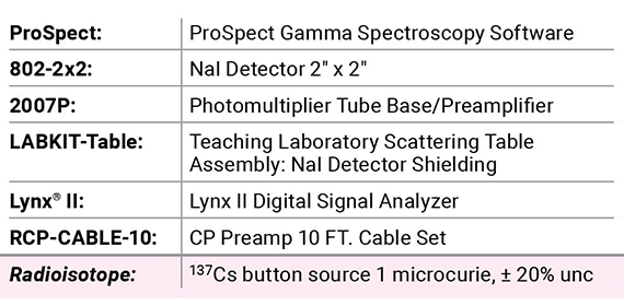
Equipment Required:
Theoretical Overview:
Detector and amplifier functions
The detection and analysis of charged particles, gamma rays, and X-rays is very much the same. A detector is basically a sensor which produces a signal when a particle or photon enters it. For a semiconductor device, the detector typically requires a bias voltage to provide an electric field to collect the charge produced in the detector volume. In scintillator detectors, a bias voltage is needed for operation of the photomultiplier tube. A detector that is used for spectroscopy produces a signal proportional to the energy of the photon deposited in the detector. This pulse is very weak and must be amplified and matched to the analysis equipment. Amplification is typically accomplished in two steps: a pre-amplification stage and a primary amplification stage.
The preamplifier is usually located very close to the detector, while the primary amplification, typically performed using a Multi-Channel Analyzer (MCA), may be at some distance from the detector, sometimes many meters. Different kinds of detector require particular types of preamplifiers, but the basic operating principles are generally similar.
The preamplifier integrates the detector charge pulse to produce a voltage pulse that has a rise time consistent with the response time of the detector, typically 10 – 200 nanoseconds, followed by longer decay time, ranging from several to many microseconds, which represents the discharge of the preamplifier feedback loop and is designed to reset the system for the next pulse. A transistor reset preamplifier is not discharged after every event, but only after several volts have been collected, representing dozens of individual events. While there may be differences in the discharge of the preamplifier, the basic principle still applies that the amount of voltage induced by the pulse is proportional to the amount of ionizing energy injected into the detector by the incident radiation.
While the preamplifier is designed to provide an immediate amplification of the weak detector signal and a reset of the system, this signal is typically not sufficient to be able extract a reliable energy signature of the pulse. A primary or shaping amplification stage is still required to further refine the pulse to be able to obtain the most accurate measure of the voltage. In traditional analog shaping the preamplifier pulse is passed through differentiation (CR) and integration (RC) filters to produce a semi-Gaussian shaped pulse signal suitable for digitization in an Analog-to-Digital converter.
Modern signal processing techniques involve the digitization of the signal direct from the output of the preamplifier stage. This digitized pulse can then be digitally manipulated to extract the most accurate pulse height. Digital pulse processing (DPP) allows for the development of filtering functions that are not possible through traditional analog processing. In addition, because of the early stage of digitization, DPP is generally more stable against changes in the environment, temperature and humidity, and faster than analog processing.
One common DPP implementation filtering function that gives optimum energy resolution is the trapezoidal filter. The basic principles of a trapezoidal filter consider two rolling averages of a determined number channels from the input digitized signal. The first average covers a time range determined by the trapezoidal “rise time”. The second average is taken for the same rise time, but starting at a time following the end of the rise time, as defined by the trapezoidal “flat top”.
These two time ranges are seen in the left panel of Figure 6-1. The filtered signal is then a difference of these two signals; as seen in the right panel of this figure. The trapezoidal filter can then be represented as:

where:

and:

In these equations:
Vin is the voltage input to the filter.
Vout is the voltage output by the filter.
RT is the user-defined rise time.
FT is the user-defined flat top.
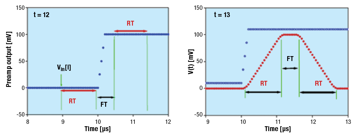
Figure 6-1: The left panel shows the trapezoidal filter parameters and the resulting output of the filter is displayed in the right panel. The blue trace represents the input signal, while the red trace represents the shaped signal.
It can be observed that the rise-time parameter represents the filter to smooth the input signal and filter out high-frequency noise that can impact the extraction of the energy signal. The flat-top parameter is usually set to be larger than the charge collection time of the detector. The rise time and flat top can be optimized to achieve the required energy resolution or throughput.
It should also be noted in the above examples, that a pure step function is used. This is a good approximation for preamplifier input pulses (on the scale of the signal rise time), but does not consider the decay time of the pulse, which is compensated for by a pole-zero correction.
Once an energy signal has been determined, there are several options available for how to utilize this signal:
Single-Channel Analysis (SCA): A digital signal is output if the energy signal is between a range of channels designated by a Lower-Level Discriminator (LLD) and Upper-Level Discriminator (ULD) range. The numbers of counts per second are typically displayed.
Multi-Channel Scaling (MCS): Similar to the SCA mode, but the data are recorded in a time histogram in which successive count rates are recorded.
Pulse-Height Analysis (PHA): Energies are recorded in an energy histogram in which pulse heights are categorized by channel and the number in each channel represents the number of times a particular pulse height was recorded within the given measurement time.
Multi-Spectral Scaling (MSS): This is similar to PHA mode, but an energy histogram is saved at short time intervals as defined by the system dwell time.
Time-Stamped List Mode (TLIST): In this mode, the time that an event occurs, to within 100 ns, is recorded along with the energy of the event. These data are stored as a list of time-energy pairs that can later be processed into any of the above four types of data. While this is the most general of the data storage options, this also uses the greatest amount of memory.
Experiment 6 Guide:
Effect of rise time and flat top
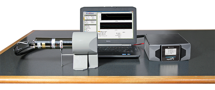
1. Connect the NaI(Tl) detector to the Lynx II DSA via the 2007P preamplifier and connect the Lynx II DSA to the PC either directly or via your local network. See Figure 6-2.
2. Place the 137Cs source in front of the detector.
3. Open the ProSpect Gamma Spectroscopy Software and connect to the Lynx II DSA.
4. Configure the MCA settings as recommended in Experiment 1.
5. Use the software to apply the recommended detector bias to the NaI(Tl) detector.
6. On the MCA settings tab, start the Digital Oscilloscope (DSO) feature of ProSpect software to view the analog input signal.
7. Set the analog trace to ADC to view the analog input signal.
8. Note how long it takes the signal to rise to its maximum and then how long it takes to fall back to the original baseline.
9. With the DSO, set the analog trace to Energy to view the digital trapezoidal figure.
10. Measure the RT and FT on the DSO.
11. On the MCA settings tab under filter settings read the RT and FT. Confirm that these match the values from step 10.
12. Change the RT setting. Record the actual rise time on the DSO.
13. Change the FT setting. Record the actual flat top on the DSO.
14. Set RT and FT back to the original values.
Effect of optimizing rise-time and flat-top settings
1. On the Acquisition setting tab of the ProSpect software, set the acquisition mode to PHA mode.
2. Set the coarse and fine gain such that the full-energy peak is close to the center of the spectrum.
3. Adjust the energy calibration such that the photopeak is about 662 keV. Please note that during this section of the experiment, the spectrum may shift from the energy calibration, and so reported values should be considered carefully.
4. On the MCA settings tab, filter settings, set a 0.6 µs RT and a 0.1 µs FT.
5. Clear the spectrum.
6. Acquire spectrum for one minute (count for longer if there is less than 3000 counts in the peak).
7. Create a Region of Interest (ROI) around the full-energy peak. Using the tooltip, record the FWHM, FWTM and centroid of the peak.
8. Change RT from 0.6 µs to 3.0 µs in increments of 0.6 µs and repeat steps 5 through 7.
9. Change FT from 0.1 µs to 1.1 µs in increments of 0.2 µs and repeat steps 5 through 8.
10. For each flat-top setting plot the energy resolution in percent, FWHM/centroid *100, versus rise time. This will remove dependency from the energy calibration and is standard practice for reporting energy resolution of scintillator detectors.
11. Determine which combination of RT and FT produces the lowest (i.e. best) energy resolution. Set RT and FT to these settings.
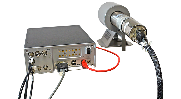
Figure 6-2: Cable connections
Single-Channel Analyzer (SCA)
1. On the Acquisition setting tab of the ProSpect software, set the acquisition mode to PHA mode.
2. Set the amplifier gain such that the full-energy peak is close to the center of the spectrum.
3. Clear the spectrum.
4. Acquire spectrum for one minute (count for longer if there is less than 3000 counts in the peak).
5. Make a Region of Interest (ROI) around the peak.
6. Record the peak area, total peak counts and the live time. Also record the lower and upper channels of the ROI.
7. Select Single Channel Analyzers under the MCA settings options menu.
8. Compute the LLD by taking the lower ROI channel, dividing by the full channel range (2048), and multiplying by 100. The converts the lower ROI channel to a percentage of the full range which is the required LLD input. Set the LLD to this value.
9. Compute and set the ULD in a similar manner as step 8, but with the upper ROI channel.
10. Select the Enable checkbox to start the SCA acquisition. Open the Time Series viewer from the MCA settings tab and record the SCA count rate, i.e. counts/sec. The count rate is displayed as the mean in the statistics box.
11. Compare this count rate to the total peak count rate in the PHA analysis in Step 6.
12. Before continuing, be sure to deselect the Enable checkbox on the SCA dialog.
Multi-Channel Scaler (MCS)
1. On the Acquisition setting tab of the ProSpect software, set the acquisition mode to PHA mode.
2. On the MCA setting tab of the ProSpect software set the Standard Conv Gain to the maximum value allowed by your MCA.
3. On the MCA settings tab of the ProSpect software and change the “MCS Conversion Gain” to the same value as the “Standard Conversion Gain”.
4. On the MCA setting tab of the ProSpect software adjust the “Coarse Gain” and “Fine Gain” such that the full-energy peak is close to the center of the spectrum.
5. Clear the spectrum. NOTE: do not change the gain once you have set it.
6. On the Acquisition setting tab of the ProSpect software, set the Preset Live time to 60 seconds.
7. Press Start and acquire the spectrum. Make sure the full-energy peak has more than 3000 counts. Adjust the Preset Live time if there are less than 3000 counts in the full-energy peak.
8. Record the total number of counts in the spectrum, hover over the deadtime bar for a tooltip or make an ROI of the full spectrum.
9. Clear the spectrum.
10. On the Acquisition tab of the ProSpect software, change the Acquisition Mode from PHA to MCS.
11. On the Acquisition tab, enter the dwell time, which is the counting time for each memory location (channel). Select a dwell time such that the total acquisition time is comparable to the acquisition time in Step 6. Remember that for the MCS mode, the total acquisition time will be equal to the total number of channels (which is given by your MCS conversion gain setting) multiplied by the dwell time (assuming a single sweep).
12. On the “Preset Options” select “Sweeps”. Enter the Preset Limit for the sweep to 1.
13. On the Disc Mode, select “MCS Fast Discriminator”.
14. Press Start to acquire the spectrum.
15. Record the total number of counts in the MCS spectrum.
16. Compare MCS counts to total number of PHA counts from Step 7, remember to correct for different count times.
Multi-Spectral Scaling (MSS)
1. On the Acquisition setting tab of the ProSpect software, set the acquisition mode to PHA mode.
2. On the MCA setting tab of the ProSpect software set the Standard Coarse Gain to the maximum value allowed by the MCA.
3. On the MCA setting tab of the ProSpect software adjust the Coarse and fine gain such that the full-energy peak is close to the center of the spectrum.
4. Clear the spectrum. NOTE: Do not change the gain once you have set it.
5. Go on the Acquisition setting tab of the ProSpect software and set the Preset Live time to 60 seconds.
6. Press Start and acquire the spectrum. Make sure the full-energy peak has more than 3000 counts. Adjust the Preset Live time if there are less than 3000 counts in the full-energy peak.
7. Make a Region of Interest (ROI) around the peak.
8. Record the net peak area and total peak area. Also record the lower and upper channels of the ROI.
9. Clear the spectrum.
10. Go to the Acquisition tab of the ProSpect software and change the Acquisition Mode from PHA to MSS. Set the Preset to Live and for the Preset Limit enter 10 seconds.
11. Go to the Spectrogram tab and set the “Data to View” to MSS Buffer and the “Number of Datasets” to 8.
12. Start acquisition and continue counting until the total acquisition time is the same as the PHA spectrum in Step 6. Remember that for MSS the total acquisition time is equal to the number of data sets measured multiplied by the preset live time.
13. On the Spectrogram tab of the ProSpect software, use the mouse and click and drag on the spectrogram plot to move through each of the MSS spectra.
14. In each MSS spectrum, record the number of peak counts in the same ROI as the PHA analysis.
15. Add the peak counts from all the MSS spectra together and record them.
16. Compare total of the MSS peak counts to the PHA peak counts.