To demonstrate the procedure for measuring the efficiency of a NaI and a HPGe detector as a function of gamma-ray energy.
To introduce the concept of efficiency calibration.
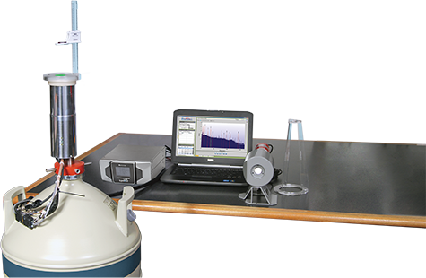
Equipment Required:
Theoretical Overview:
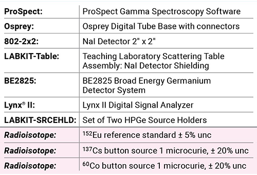
A radioactive source emits a certain number of photons (gamma radiation) and the detector (e.g., NaI scintillation or HPGe detector) is used to detect these photons. The number of photons emitted by the radioactive source is always larger than the number of photons observed by the detector, and the ratio of the number of photons detected or observed by the detector with respect to the number of photons emitted by the source is known as the detection efficiency. The detection efficiency, ε, can be stated as follows:
where: Nmeas is the number of counts (photons) observed by the detector. Nemit is the number of photons emitted by the source.
In the majority of applications the full-energy peak efficiency is of interest; in that case the Nmeas is the number of counts in the full-energy peak and Nemit is the number of photons emitted for a specific energy.
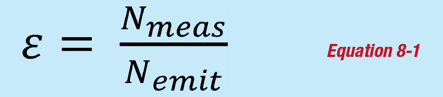
Figure 8-1: Decay scheme of 137Cs.
The number of counts observed in the detector depends largely upon the characteristics of the detector such as size, atomic number and density. The number of counts observed also depends on the activity of the source, the source-to-detector distance and the materials between the source and the detector. The activity of the source defines the rate of decay (or disintegration) of the source; this is usually expressed in units of becquerel or Curie. One becquerel is equivalent to one disintegration per second while one Curie is equivalent to 3.7 x 10¹⁰ disintegrations per second. For most nuclei, the number of photons emitted per second for a certain energy is not the same as the number of disintegrations per second, it is usually less. There may be different decay paths in the daughter nucleus and the transition of interest might be bypassed by other transitions. The total number of gamma rays emitted from a disintegration can be larger than one. Other decay mechanisms such as internal conversion compete with the gamma-ray emission. The parameter used to describe the number of gammas per disintegration for a gamma-ray energy is known as the intensity or yield. The number of counts expected can be defined as shown in Equation 8-2.
where: A is the activity in disintegrations per second (or Bq). Y is the gamma-ray yield. t is the time in seconds.
The activity of the source is usually specified with respect to a certain date. The current activity at the time of experiment has to be decay corrected using Equation 8-3.
where: A is the current activity. A0 is the activity on the reference date. t is the time elapse since the reference date. t1/2 is the half-life of the nuclide under consideration.
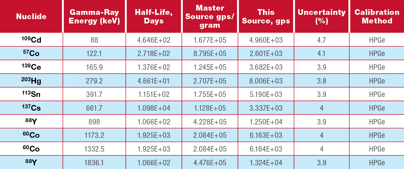
All traceable radioactive sources have source certificates, which provide the source activity stated in becquerel or Curie on the date the activity was measured. However, some certificates state the emission rate in gammas per second, which implies that the yield or intensity has been factored into the values given. This is common with mixed-gamma sources, as is shown in Table 8-1.
Table 8-1: Typical source certificate for a mixed gamma source.
Efficiencies can be referred to as absolute, intrinsic, or relative. Absolute efficiency is the ratio of the total number of photons detected to the number of photons emitted by the source. Intrinsic efficiency is the ratio of the number of photons detected to the number of photons incident on the detector surface. Absolute and intrinsic efficiencies can be expressed as the full-energy peak efficiency which takes into consideration only the photons which result in counts in the full-energy peaks. Often, Germanium detector efficiencies are expressed as relative efficiencies. This is the efficiency relative to a 60Co source (using the 1332 keV peak) measured with a 3"x 3" NaI(Tl) detector at a distance of 25 cm from the detector.
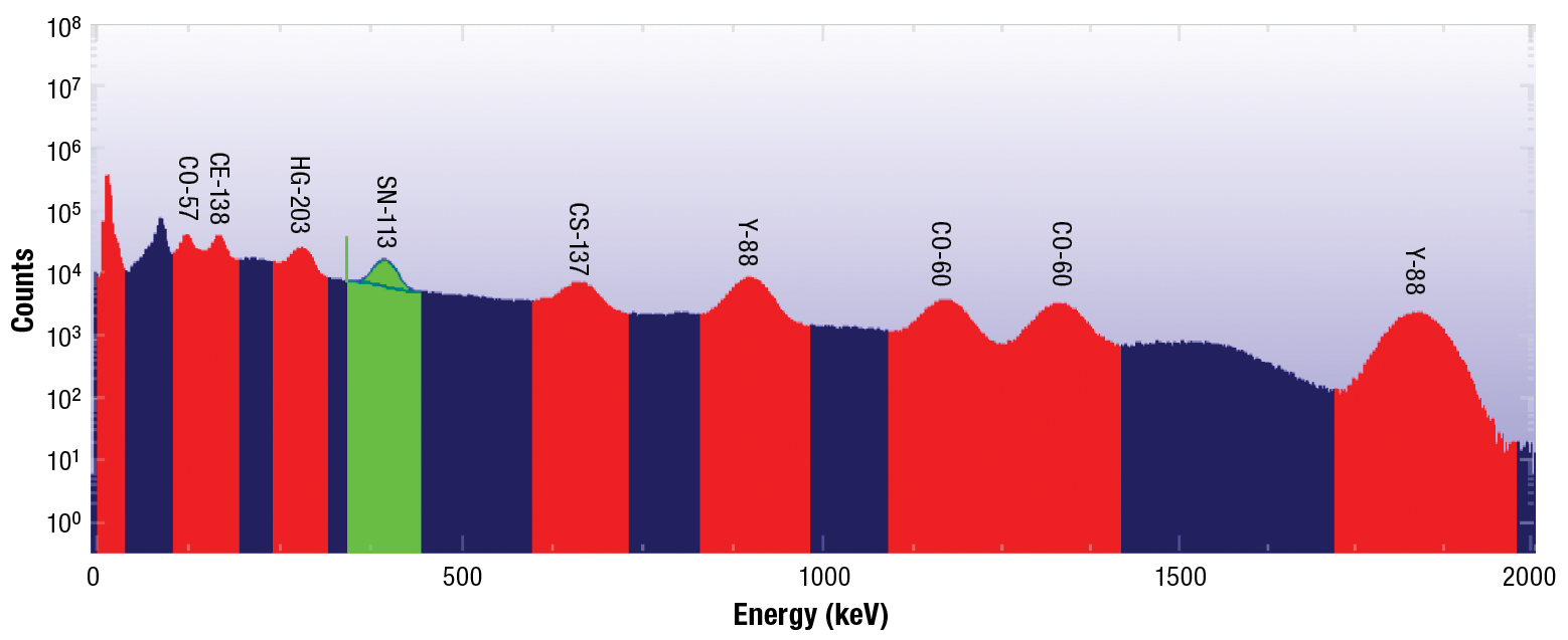
Figure 8-2: Typical NaI spectrum for a mixed gamma source.
Experiment 8 Guide:
Using 2" x 2" NaI detector
1. Place the 152Eu reference standard at a distance of about 20 cm from the surface of a 2"x 2" NaI detector.
2. Configure the MCA settings as recommended in Experiment 1.
3. Adjust the coarse and fine gain of the MCA such that the 1408 keV peak is visible in the high-energy region of the spectrum.
4. Acquire data, ensuring that at least 10 000 counts are achieved in several of the major peaks throughout the spectrum. By referring to Experiment 2 if needed, perform an energy calibration.
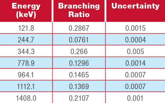
5. Measure the net peak area and uncertainty for each of the major peaks listed in the certificate file. For each gamma-ray peak, use Equation 8-1 to determine the efficiency. Also calculate the uncertainty in the efficiency (use Reference 4 on Page 77 if needed). Note if counts (rather than counts per second) is to be used for this calculation (as per Equation 8-1) then the gamma-ray emission rates in the certificate file should first be converted to number of gamma rays emitted during the acquisition (by multiplying by the time of the acquisition). The photon intensities are provided in Table 8-2 for easy reference.
Table 8-2: Branching ratios for major 152Eu gamma rays.
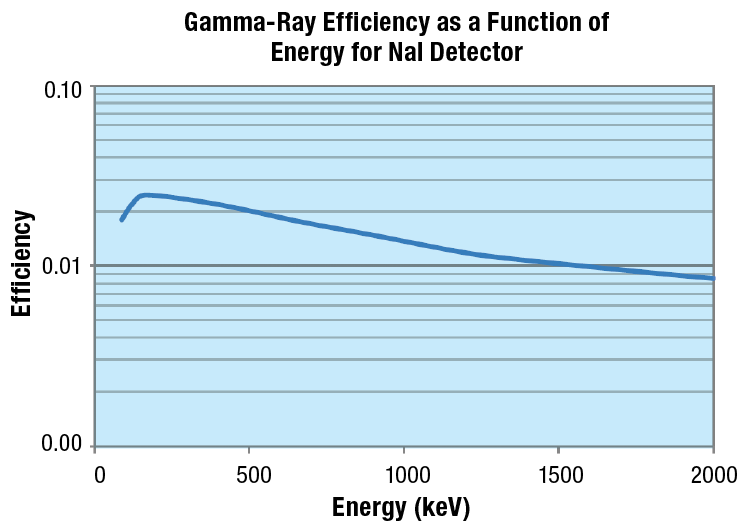
6. Plot the efficiency (and uncertainty) against energy in Microsoft Excel or other program. The result should be similar to Figure 8-3. Comment on the shape of the curve.
Figure 8-3: Representative efficiency of NaI detector as a function of energy.
Using the HPGe detector
The determination of the efficiencies using the HPGe detectors is similar to that of the 2"x 2" NaI detector.
The main difference in the results obtained is that the resolution of the HPGe detector is much better than that of a NaI detector. Typical resolution of a HPGe detector is less than 0.2% while it is about 7.5% for a NaI detector.
1. Ensure that the Lynx II DSA (with the HPGe detector connected) is connected to the measurement PC either directly or via your local network.
2. Using the adjustable source holder, place the 152Eu reference standard at a distance of about 20 cm from the endcap of the high-purity germanium detector. Record this distance. Remove the plastic cap from the detector before counting.
3. Open the ProSpect Gamma Spectroscopy Software and connect to the Lynx II DSA.
4. Configure the MCA as recommended in Experiment 7 for a HPGe detector.
5. Use the software to apply the recommended detector bias to the HPGe detector.
6. Set the PHA conversion gain to 32768 channels.
7. Adjust the coarse and fine gain of the MCA such that the 1408 keV peak is visible in the upper part of the spectrum.
8. Acquire data, ensuring that at least 10 000 counts are achieved in several of the major peaks throughout the spectrum. Energy calibrate the system, referring the Experiment 1 if needed.
9. Measure the net peak area and uncertainty for each of the major peaks listed in Table 8-2. For each full-energy peak, use Equation 8-1 to determine the efficiency. Also calculate the uncertainty in the efficiency (use Reference 4 on Page 77 if needed). Note if counts (rather than counts per second) is to be used for this calculation (as per Equation 8-1) then the gamma-ray emission rates in the certificate file should first be converted to number of gamma rays emitted during the acquisition (by multiplying by the time of the acquisition). The photon intensities are provided in Table 8-2 for easy reference.
10. Plot the efficiency (and uncertainty) against energy in Microsoft Excel or other program. Compare the results to the efficiency determined from the NaI measurement.
11. Remove the 152Eu reference standard and replace with the 60Co source at the same distance. Count until at least 10 000 counts are in each of the two primary peaks. Using Equations 8-2 and 8-3 and by interpolating using the efficiency curve calculated in Step 10, determine the activity of the 60Co source. How does this compare against the 60Co source certificate?
12. Repeat Step 11 with 137Cs source. Again, how does this compare against the activity on the source certificate?
13. Using one of the sources, place the source at a distance of 10 cm and 25 cm. For each position, count until there are about 10 000 counts in the primary peaks. Calculate the efficiency curve for each geometry. How do they compare? Do they demonstrate that efficiency is proportional to the inverse of the distance squared?