To use the technique of coincidence detection and demonstrate the basic principles of coincidence measurements.
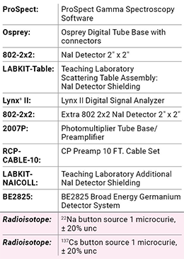
Equipment Required:
Theoretical Overview:
Coincidence measurements are an important tool in the detection of ionizing radiation for a wide range of applications. Many nuclear processes produce two photons simultaneously, while other processes produce two or more photons in quick succession. In such cases, it is possible to study the temporal and angular correlations between the two photons by setting up a coincidence detector system. These emissions can occur simultaneously or within a time period that is very short compared to the time resolution of the detection system. For example, decay by beta emission to a daughter nucleus, which in turn decays by gamma emission, produces the beta particle and the gamma ray at essentially the same time. Similarly, one nucleus may emit several gamma rays in cascade, which are effectively simultaneous because the delay between the events is short. Delays of 10-9 seconds are common.
In nuclear physics applications, coincidence systems are used to detect and identify weak detection signals or to distinguish a physics signal from background signals, as is done in Compton suppression or cosmic veto systems. In high-energy or particle physics, detection systems consisting of thousands of detectors and electronics channels are all operated in coincidence when two accelerated beams collide to search for newly formed particles or new decay pathways.
Time-coincidence measurements
In addition to radiation detector characteristics such as efficiency or energy resolution, time resolution is important to measure. This is required to determine the time dependence of nuclear decays as discussed previously. It reflects the ability to measure the arrival time of the incident particle or the time of a specific interaction and its associated signal. The time resolution of a specific detector depends on several parameters such as signal shape called “walk time” and signal noise called “jitter time”.
In some cases the actual time difference between the two events can be measured, but in many cases it is only necessary to determine that the events are correlated in time.
The determination that two nuclear events occur at the same time is made electronically with a coincidence system. This unit operates on standardized pulses and determines whether events occur within a certain time interval, called the resolving time. The standard pulses from any single channel analyzer are used as input, with one input from each detector.
The number of coincidences that are real, not random, is determined by the physics of the decay and the solid angles and efficiencies of the detectors. These are the true coincidences.
In some experiments, the number of coincidences is the only information needed. Often, however, the coincidence signal is used to open the linear gate in a multichannel analyzer so that a spectrum is acquired under coincidence conditions.
This experiment has three separate parts which use the coincidence technique in different ways.
γγ Angular correlations
The angular correlation of two gamma rays, γ1 and γ2 may be defined as the probability of γ2 being emitted at an angle relative to the direction of γ1. The emission of gamma rays from excited nuclei can be treated mathematically as the classical radiation of electromagnetic energy from a charged system. The electric field can be expanded in vector spherical harmonics, corresponding to the various multipoles of the charge distribution. The shape of the angular distribution of the radiation with respect to the radiating system is uniquely determined by the order of the multipole.
In nuclear systems, the order of the multipole depends upon the angular momentum numbers and the parities of the initial and final states involved in the transition. Thus, if all nuclei in a radioactive sample could be oriented so that their nuclear angular momenta were aligned, the shape of the angular distribution of gamma rays could be used to determine the multipolarity of the transition.
However, nuclei are randomly oriented. Very strong magnetic fields at low temperature could be used to provide orientation, but a simpler method is to use coincidence technique for cases in which two or more gamma rays are emitted in cascade. The first gamma ray establishes the direction of the spin axis of the nucleus; hence the second gamma ray will have a definite distribution with respect to this axis. One needs only to measure the angular correlation for the two gamma rays and compare it with the tabulated values for various multipolarities.
In nuclear physics experiments the angular correlation is measured between two gamma rays, which are emitted almost simultaneously in the cascade from the decay of a radioactive nucleus. The gamma rays are detected using two NaI scintillation counters in which the height of the electronic output pulses is proportional to the incident gamma ray energies. By pulse height selection, in “single channel analyzer mode”, one counter will be used to record γ1 and the other γ2. The counting rate of each counter, Ri, for detecting its selected gamma ray is given by:
where:
N0 is the number of decays per second in the radioactive source. ei is the efficiency of the detector. Oi is the geometrical solid angle subtended by the detector. In the absence of the angular correlations, the true rate of detected gamma-ray coincidences is:
The random coincidence rate between a gamma ray detected in Detector 1 and a gamma ray detected in Detector 2 is:
where Δt is the resolving time of the coincidence counting system between the two detectors. If both detectors are set to respond to both gamma rays, the counting rate in each detector is the sum of counting rates for different gamma rays.
Experiment 9 Guide:
Time-coincidence measurements using TLIST acquisition mode NaI-NaI coincidences
Energy calibration
1. Use two NaI Detectors (one connected via an Osprey unit and the other with the 2007P Preamp and Lynx II DSA) connected to the measurement PC either directly or via your local network.
2. Open the ProSpect Gamma Spectroscopy Software and connect to both MCAs.
3. Configure both MCAs as recommended in Experiment 1 for configuration to a NaI detector.
4. Select the High Voltage Settings on the Detector tab on the ProSpect software to apply the recommended high voltage on both detectors.
5. Place the 22Na source between the two detectors in a close geometry.
6. Set the Conversion gain on the MCA tab of the ProSpect software to 2048 channels for both MCAs.
7. Adjust the coarse and fine gain settings on the MCA tab of the ProSpect software on both MCAs such that the 1275 keV full-energy peak is in the upper part each spectrum.
8. Click on Start (on the top of each Spectral Display) to start accumulating the two spectra. Use a count time such that there is at least 10 000 counts in the full-energy peak.
9. Perform an energy calibration using the 511.0 and 1274.5 keV peaks of 22Na, referring to Experiment 1 if necessary.
Decay spectra
10. On the acquisition tab set the acquisition mode to TLIST mode. The TLIST mode allows acquisition of event data which provide the energy and time for each event.
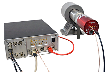
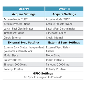
11. Set the two devices up according to Table 9-1. Note that the external sync setting needs to be applied first. Connect the Sync BNC connector on the Lynx II DSA rear panel to the GPIO input channel 1 of the Osprey unit. See Figure 9-1. (If necessary, utilize a 50 ohm terminator to reduce reflections.)
12. Press Control-Start to begin acquisition simultaneously on both devices.
Figure 9-1: Cable configuration for synchronization of Lynx II and Osprey DSAs.
13. Ensure that both detectors go into waiting mode (blue backgrounds on the datasource thumbnails). Rapidly (before the 20 second timeout is reached), switch the Lynx II DSA External Synchronization from Slave to Master B.
14. Ensure that both detectors begin acquiring data (PHA data appears in the display and both backgrounds turn green in the datasource thumbnail view).
15. Acquire data for around 5 minutes, press Control-Stop to stop both MCAs from acquiring data and save the PHA data. The TLIST data is saved automatically during the acquisition.
Table 9-1: Settings of synchronized TLIST mode acquisition with an Osprey and Lynx II DSA
Analysis
16. To analyze the TLIST mode data and see the results of the coincidence measurement use the application called ProSpect Data Scanner (downloadable from Mirion website www.mirion.com). Follow the steps below to run the ProSpect Data Scanner.
17. Select the folder of interest, where the data are stored.
18. Select the Pre-Scan option to sort the events by the time stamp. Note that for each file the elapsed and the live time is displayed. Additionally, the total number of events in PHA and TLIST mode data and the elapsed real and live times for the TLIST mode data file are displayed.
19. Enter the energy calibration equations for both detectors, found on the energy calibration tab. Select Energy-Scan to reconstruct the energy spectra for both devices from the TLIST events.
20. To ensure the time correlations between the events can be observed, set a gate around the 511 keV full-energy peak.
21. Select the Time-Scan to generate the time coincidence spectrum. The display spectrum will show the time correlation between the events recorded in both detectors.
22. Comment on the time-correlated spectrum.
NaI-HPGe coincidences
Energy calibration
1. Connect the Lynx II DSA (with the HPGe detector connected) to the measurement PC or via your local network using the Ethernet connection.
2. Connect the Osprey unit (with the NaI(Tl) detector connected) to the measurement PC either directly or via your local network.
3. Open the ProSpect Gamma Spectroscopy Software and connect to the Lynx II and Osprey units.
4. Configure the NaI detector as recommended in Experiment 1, and the HPGe detector as recommended in Experiment 7.
5. Select the High Voltage Settings on the Detector tab on the ProSpect software to apply the recommended high voltage on both detectors.
6. For each detector perform an energy calibration using the 511.0 and 1274.5 keV peaks of 22Na, referring to Experiment 1 if necessary.
7. Save both spectra. Once you have set the gain and the energy calibration coefficients, do not change it, otherwise you will have to redo the calibration.
Decay spectra
8. On the ProSpect software set the data acquisition to TLIST mode. The TLIST mode allows simultaneous acquisition of event data which provide the energy and time for each event.
9. To acquire data in TLIST mode set both detectors as shown in Table 9-1.
10. After the two devices are setup as described in Table 9-1, make sure to connect the Sync BNC connector on the Lynx II DSA rear panel (add a 50 ohm terminator to prevent reflections) to the GPIO input channel 1 of the Osprey unit.
11. Select Control-Start to begin acquisition simultaneously on both devices.
12. Ensure that both detectors go into waiting mode (blue backgrounds on the datasource thumbnails). Rapidly (before the 20 second timeout is reached) switch the Lynx II DSA External Synchronization from Slave to Master B.
13. Ensure that both detectors begin acquiring data (PHA data appears in the display and both backgrounds turn green in the datasource thumbnail view).
14. Acquire data for around 5 minutes and save the data.
Analysis
15. To analyze the TLIST mode data and see the results of the coincidence measurement use the application called the ProSpect TLIST Data Scanner (downloadable from the Mirion website). Follow the steps below to run the ProSpect TLIST Data Scanner.
16. In the Search Directories tab, identify the directory with the acquired TLIST data. Press the start button to begin analyzing.
17. In the Scan Results tab, select the appropriate acquisitions and set the beginning time Range to -6000 ns, maximum time range to 6000 ns, and the Time Bins to 1000.
18. On the Analysis tab, select the two acquisitions using the Device and Acq Start tabs. Plot Energy on the X-axis and Time on the Y-axis to observe the coincident counts. Comment on the graph that is observed. Note: You can copy the graph to your clipboard for further analysis.
19. Comment on the time coincidence spectrum and compare with the spectrum acquired for the two Osprey units above.
Time-coincidence measurements using lynx II hardware gating
This section requires the following: ProSpect Version 1.1
1. Make sure the high-purity germanium (HPGe) and NaI detectors are energy calibrated.
2. Place 137Cs and 22Na sources between the two counter detectors in a closed geometry.
3. Connect the GPIO 1 unit of the Osprey digital MCA to the gate input of the Lynx II DSA.
4. For the NaI detector, open the GPIO dialog on the MCA tab of the ProSpect software and set the GPIO to the single-channel analyzer, SCA 1.
5. For the NaI detector, go to the Single-Channel Analyzer under the MCA tab of the Prospect software and Enable the SCA.
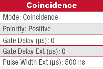
6. Go to the Acquisition tab of the Prospect software for the Lynx II unit and set the coincidence gate parameters as follows:
Table 9-2: ProSpect Settings for Step 6.
7. Launch the Digital Oscilloscope and look at the Lynx II traces. Set the trigger on the Store pulse and make sure the external gate is overlapping with the peak detect pulse. Increase the Gate Delay Ext such that the edge of the peak detected will overlap with the edge of the external gate.
8. Acquire an energy-gated spectrum in the HPGe detector. Use a count time such that there are at least 10 000 counts in each photopeak.
9. Save the spectrum.
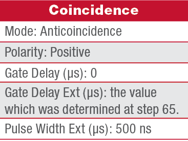
10. Set the coincidence gate settings as follows:
Table 9-3: ProSpect Settings for Step 10.
11. Acquire an energy-gated spectrum in the HPGe detector. Use a count time such that there are at least 10 000 counts in each photopeak.
12. Save the spectrum.
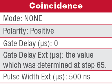
13. Set the coincidence gate settings as follows:
Table 9-4: ProSpect Settings for Step 13.
14. Acquire an energy-gated spectrum in the HPGe detector. Use a count time such that there are at least 10 000 counts in each photopeak.
15. Save the spectrum.
16. Plot the energy spectra acquired with different coincidence-gating conditions and compare the number of counts in the photopeaks for the different gating conditions.