Lab Experiment 4: Compton Scattering
Powered by Lab-Kits for Nuclear Science Experiments
Purpose:
- Demonstrate how the gamma-ray energy varies following Compton scattering.
- Demonstrate the possible range of scattered gamma-ray energies.
Equipment Required:
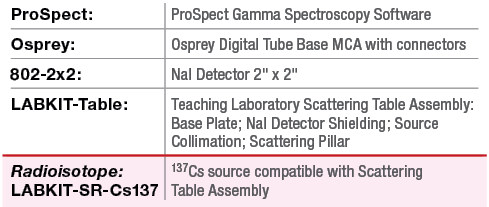
Theoretical Overview:
Scattered energy as a function of angle
As previously discussed in Experiment 1, in Compton scattering a photon of energy Eγ and momentum Eγ/c scatters inelastically from an electron of mass m0c2. Some of the energy of the photon is transferred to the electron, and the photon is scattered through an angle θ with reduced energy Eγ′.
The Compton scattering formula can be written as:
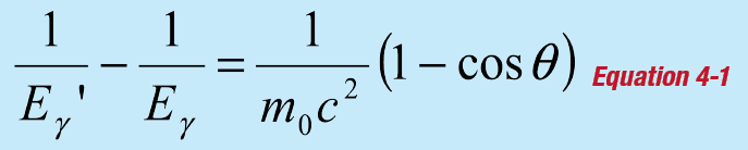
This may be rearranged as the equation for a straight line:
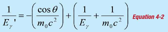
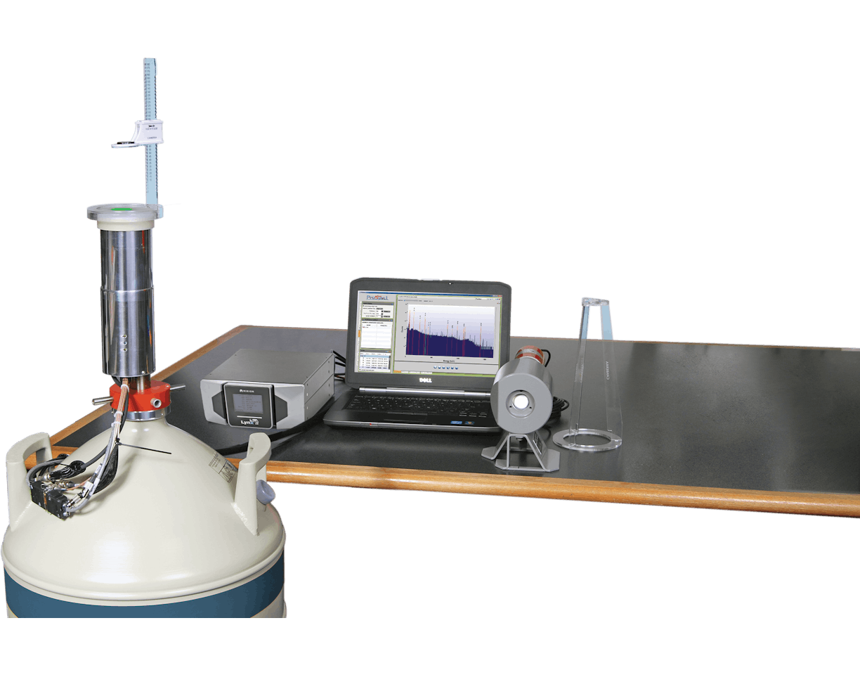
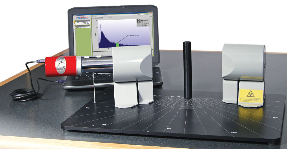
In this experiment Eγ is measured as a function of θ for incident gamma rays of 662 keV from a 137Cs source. Figure 4-1 illustrates the experimental setup, where the detector is positioned at about θ = 40°.
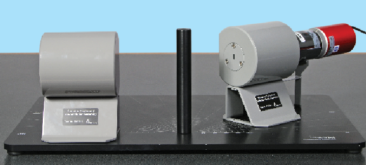
Figure 4-1: Collimated 137Cs source and NaI detector positioned on the scattering table.
Note: During this experiment you should work in keV, where the mass of the electron is 511 keV/c2.
The expected energies are shown in Figure 4-2:
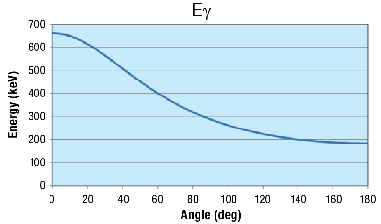
Figure 4-2: The energy of the Compton-scattered photon as a function of scattering angle for an initial photon energy of 662 keV.
Angular distribution
The scattering probability as a function of angle is called the differential cross section, and for Compton scattering it is given theoretically by the Klein-Nishina formula (the units are square meters per steradian, m2/sr):

where:
r0 = 2.82 x 10⁻¹⁵ m, the classical electron radius, and for 137Cs
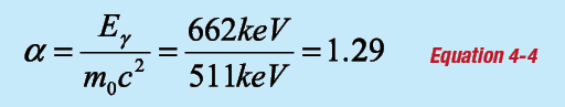
A plot of the differential cross section, dσ/dΩ, is shown in Figure 4-3. The units are barns per steradian, b/sr , where 1 barn = 10-28 m2.
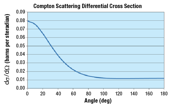
Figure 4-3: The differential cross section of Compton scattering for a photon energy of 662 keV.
Experiment 4 Guide:
1. Use the ProSpect software to connect to the detector. Configure the MCA settings and bias voltage as recommended in Experiment 1. Make sure that the detector is correctly calibrated for energy.
2. Ensure the collimated 137Cs source fixture is aligned at the 1800 mark and is pointing toward the aluminum scattering pillar. During this experiment, keep the source fixture fixed at this location. Caution: Be sure to be aware of your surroundings. Do not have the source pointed at yourself or any other people working in the laboratory.
3. Place the detector with the collimated detector shielding on the scattering table. Starting with the 00 marking, orientate the detector assembly toward the aluminum scattering pillar. Acquire a spectrum until a noticeable peak is visible. Note: To increase the count rate, you can complete this experiment without the add-on detector collimator slit. For better angular resolution, use the detector collimator slit in the vertical orientation and extend the counting time until good statistics are achieved.
4. Repeat Step 3, moving the detector assembly to different angles up to 1600 degrees.
5. For each measurement determine the centroid energy of the scattered peak.
6. In a spreadsheet, plot the energy of the scattered peak as a function of angle and compare the results with Figure 4-1.
7. Plot the reciprocal of the scattered gamma-ray energy (1/E′ ) as a function of ( 1 - cos θ ). Use the graph and Equation 4-1 to determine the original gamma-ray energy and the rest mass of the electron. Check that these match the values provided above.
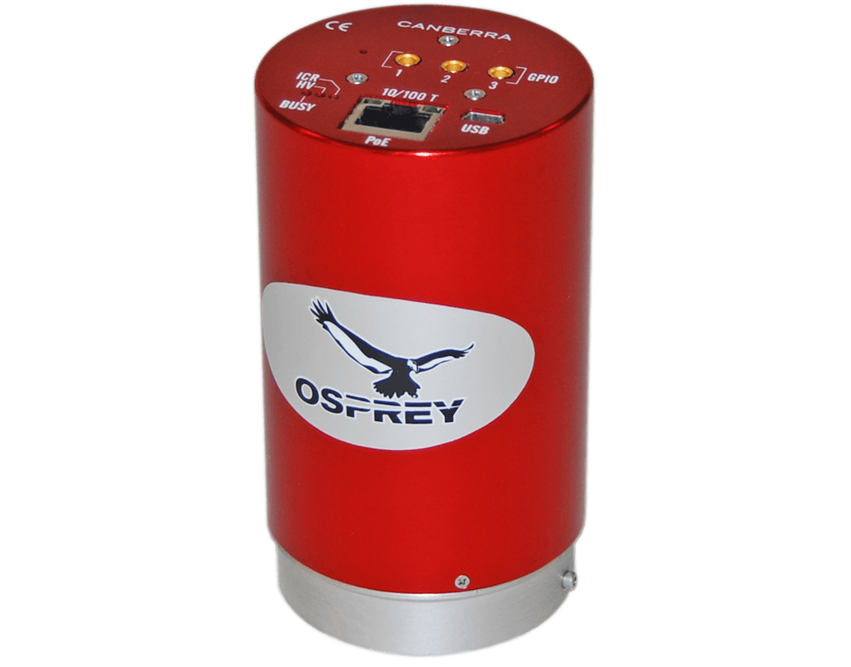
Osprey®
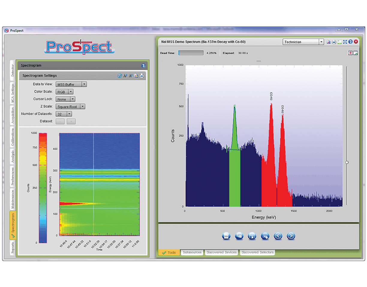
ProSpect®
Do you have a question or need a custom solution? We're here to help guide your research.